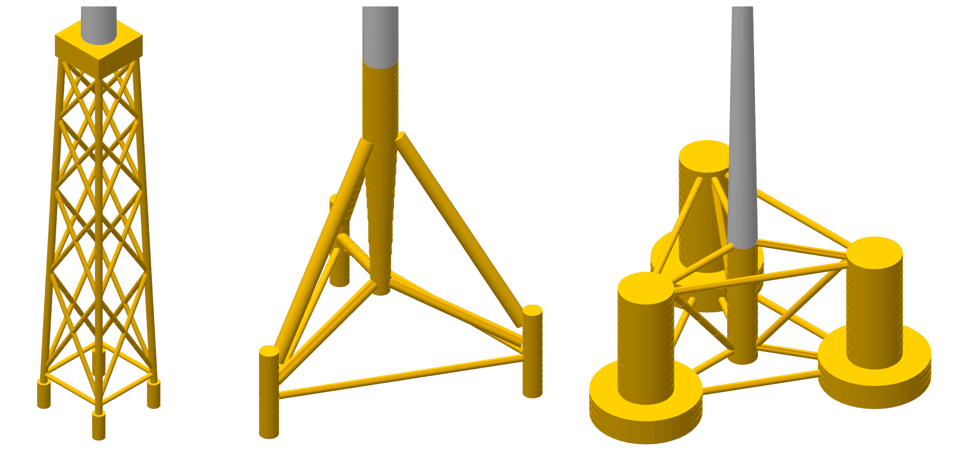
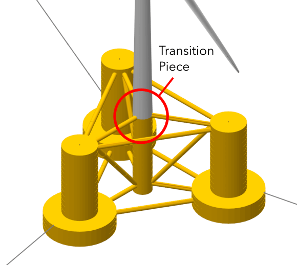
Fig. 118 Three different substructures (in yellow) connected to the tower bottom (grey).
Optionally, a substructure definition can be added to the structural model of a wind turbine in QBlade. The substructure definition can fulfill several different roles. Below a few typical applications of substructure definitions are given:
Lattice towers: The substructure can be used to model the turbine tower with greater freedom as the standard tower file, which can only model tubular, straight towers, for instance by explicitly defining a lattice tower structure in the substructure file.
Floaters and moorings: The substructure can be used to define the floater of a floating offshore wind turbine (FOWT). This requires that the floater is modeled both hydrodynamically (Morison or Potential flow) and structurally (flexible or rigid) within the substructure definition. The substructure definition is also used to define the mooring system which keeps the floater in place.
Soil modeling: In the substructure file a p-y curve can be defined to model nonlinear soil dynamics, both onshore or offshore.
Multi-rotor assemblies: The substructure definition is also used to define the substructure of a multi-rotor assembly, with an arbitrary number of rotors.
To add a substructure to a turbine definition you need to add the filename of the substructure definition followed by the keyword SUBFILE anywhere within the main structural input file.
It is possible to connect the substructure either to the tower bottom, torquetube bottom or directly to the rotor nacelle assembly (RNA) of a turbine definition. If the main structural input file contains a TWRFILE the transition piece of the substructure (TP_INTERFACE_POS) is automatically connected to the tower bottom. If the substructure contains no TWRFILE keyword the transition piece is connected to the rotor nacelle assembly (RNA).
When it comes to modeling the hydrodynamics and structural dynamics of an offshore substructure, there are several options to consider. This section is meant to give an overview on how different aspects can be modeled:
The substructure is typically composed of interconnected members and joints (see Substructure Topology). These members can be modeled as either flexible (with associated stiffness, mass, etc.) or rigid (with or without mass). If the members have nonzero mass properties, the substructure’s mass and inertia are explicitly included. Alternatively, the complete substructure’s mass can be represented using a 6x6 mass matrix, known as lumped mass (see Lumped Mass, Inertia and Hydrodynamic Forces).
Similar to mass and inertia, substructure buoyancy can be modeled explicitly or in a lumped linearized manner. Explicit modeling involves enabling the buoyancy calculation for each member based on its submerged part in the SUBMEMBERS table (see Substructure Members). Explicit buoyancy applies buoyancy forces locally to each member. In the lumped approach, a 6x6 hydrodynamic stiffness matrix is defined to represent the substructure’s buoyancy restoring forces and moments (see Lumped Mass, Inertia and Hydrodynamic Forces). This linearized hydrodynamic stiffness matrix is valid for small rotations and translations of the substructure.
The hydrodynamic forces acting on a substructure can be evaluated by means of linear potential flow theory or the Morison equation. When the Morison Equation is used (see Morison Equation (Strip Theory) Modelling) Morison coefficients are assigned to each substructure member and the resulting forces (based on local wave and floater kinematics) are applied locally to each member. Alternatively, a linear potential flow solver (such as WAMIT, NEMOH, or ANSYS AQWA) can generate databases representing lumped hydrodynamic forces acting on the substructure (see Linear Potential Flow Modelling). Furthermore, it is also possible to assign lumped 6x6 hydrodynamic linear or quadratic drag and added mass matrices (see Lumped Mass, Inertia and Hydrodynamic Forces).
It is possible to combine different approaches mentioned above. A common mix involves using linear potential flow hydrodynamics along with the Morison equation to account for viscous hydrodynamic drag. If obtaining distributed loads for substructure components is important, hydrodynamic forces should be distributed as well (Morison equation with explicit buoyancy modeling), and the substructure members should be modeled as flexible elements. By carefully selecting and combining these modeling options, a comprehensive understanding of the hydrodynamics and structural dynamics of an offshore substructure can be achieved.
Feature
Explicit Modeling
Lumped Modeling
Mass
Defined by
substructure’s
members.
Represented via a
6x6 mass matrix.
Buoyancy
Calculated for each
member based on
submerged parts.
Represented by a
hydrodynamic
stiffness matrix.
Hydrodynamics
Distributed forces
via Morison
coefficients.
Lumped forces from
external potential
flow databases.
As with the other structural definition files, the substructure is defined by a series of keywords that are recognized by QBlade when creating the turbine. The format is the same as with the other structural file definitions:
A parameter is defined by its value followed by the parameter Keyword:
<Value>KEYWORD, for parameters defined by a single values.
Value KEYWORD
A table is identified by its Keyword and the row and column count of the subsequent ASCII values, which need to separated by space(s) or tab(s).
An example of a table with two rows and three columns is shown below.
KEYWORD <new line> <Header> <new line> <Values> for parameters defined by a table. The <Header> <new line> part is only optional and can be omitted.
There is no particular order in which these keywords and the associated data tables should be placed. The only exception is when defining tables. When a table is defined by a keyword, it should be immediately followed by the
table header (optional) and the table content.
The following keywords can be used to define different properties and modeling options for the substructure.
ISFLOATING
[bool] A flag that determines if the substructure is floating of bottom-fixed. If the structure is bottom-fixed the joint coordinates (see SUBJOINTS below) are assigned in a coordinate system with its origin placed at the seabed. For floaters, the origin is placed at the mean see level (MSL) and marks the floater’s neutral point (NP)
true ISFLOATING
WATERDEPTH
[m] Sets the design water depth of the substructure, this value is only used for visualization of the turbine and the identification of flooded members during turbine setup. Note that this water depth is only for the turbine setup and is not used during the simulations. During the simulation the water depth is obtained from the simulation settings.
220 WATERDEPTH
WATERDENSITY
[kg/m^2] Sets the water density to calculate the mass of the flooded members. Note that this water density is only for the turbine setup and is not used during simulations. During simulations the water density is obtained from the simulation settings.
1025 WATERDENSITY
SEABEDDISC
[m] Sets the sub-discretization length for mooring lines in contact with the seabed, in [m]. A value of 1 means that when a mooring line element is in contact with the seabed the mooring element will be discretized into elements of 1m length for which the contact forces will be evaluated. The default value is 2.
1 SEABEDDISC
FIXEDFLOATER
[bool] A flag that if set to true fixes the floater to the ground (by constraining the neutral point). A fixed floater can be subjected to a prescribed motion via a Prescribed Motion File (see Turbine Events and Operation).
true FIXEDFLOATER
FIXEDRAMPUP
[bool] A flag that if set to false prevents the floater from being held fixed (at the neutral point) during the rampup. This is intended to help the floater to find its equilibrium position already during rampup. The default setting is true, e.g. the floater is held fixed during rampup.
false FIXEDRAMPUP
BUOYANCYTUNER
[-] A multiplication factor that affects the calculation of the explicit buoyancy forces. Buoyancy caused by the linear hydrodynamic stiffness matrix is not affected by this factor.
1.0032 BUOYANCYTUNER
BUOYANCYPREDICTOR
[-] Dimensionless look-ahead factor for evaluating hydrostatic pressure within a time step. Positions are predicted using velocity and acceleration before computing explicit buoyancy. Does not affect the linear hydrostatic stiffness.
Default: 0.65
Typical range: 0 … 1 (0 = no prediction, 1 = full one-step look-ahead; values >1 may destabilize)
Controls the discretization of cylindrical members during buoyancy calculations. In QBlade, buoyancy forces are determined by integrating the hydrostatic pressure over the wetted surfaces of each member, including both sidewalls and end faces. The ADVANCEDBUOYANCY parameter defines into how many circumferential strips the sidewalls of a cylindrical member are subdivided for this integration. A higher number of strips increases the geometric resolution of the buoyancy model, leading to more accurate force predictions for partially submerged or inclined members, at the cost of additional computation. The default value, if not specified, is 72 subdivisions, which provides a good balance between accuracy and performance for most applications.
200 ADVANCEDBUOYANCY
STATICBUOYANCY
[bool] An optional flag that controls for which sea level the explicit buoyancy is calculated in QBlade. If set to true, the buoyancy is considering only the mean sea level. If set to false (default), the local wave elevation at each member is used to calculate the buoyancy. When evaluating the hydrodynamics using potential a potential flow theory excitation database (USE_EXCITATION) it is recommended to enable the STATICBUOYANCY option since the hydrodynamic forces due to a change in wave elevation are already accounted for by the excitation forces. Using the instantaneous sea level for the evaluation of buoyancy in such a case would cause this part of the buoyancy force to be double-accounted for.
true STATICBUOYANCY
STATICSUBMERGENCE
[bool] An optional flag that controls which sea level is used for the wetting / submergence check of Morison elements in QBlade. If set to true, Morison elements are considered wetted (or dry) based on the mean sea level (MSL) only. If set to false (default), the local instantaneous wave elevation at each member is used for the wetting check, i.e. members can enter and leave the water depending on \(\zeta(x,y,t)\). When evaluating hydrodynamics using a potential-flow excitation database (USE_EXCITATION), it can be beneficial to enable STATICSUBMERGENCE to avoid double-accounting of free-surface effects (e.g. additional load contributions introduced by time-varying wetted length/area) that may already be represented in the excitation loads.
false STATICSUBMERGENCE
HYDROJOINTVENTED
Excludes all member end faces connected to this joint from applying the hydrodynamic pressure during buoyancy calculations. Also, no Morison loads are applied at vented nodes. This setting is used to represent joints, where no hydrodynamic forces are evaluated. In the example shown below the end face loads are not applied to the subjoints with ID’s 1 4 6 and 12 during hydrodynamic calculations. This feature is useful if the user wants to measure the internal axial loads in between two members. At the location where these loads are measured the internal joints should be set to vented.
HYDROJOINTVENTED 1 4 6 12
MARINEGROWTH
A table that allows the user to define different types of marine growth that is present in the members. In QBlade, marine growth is simulated as an additional thickness that affects the diameter of the cylindrical or rectangular element. An entry is defined by its ID number, the thickness of the growth (added to the cylinder radius) and the density of the growth.
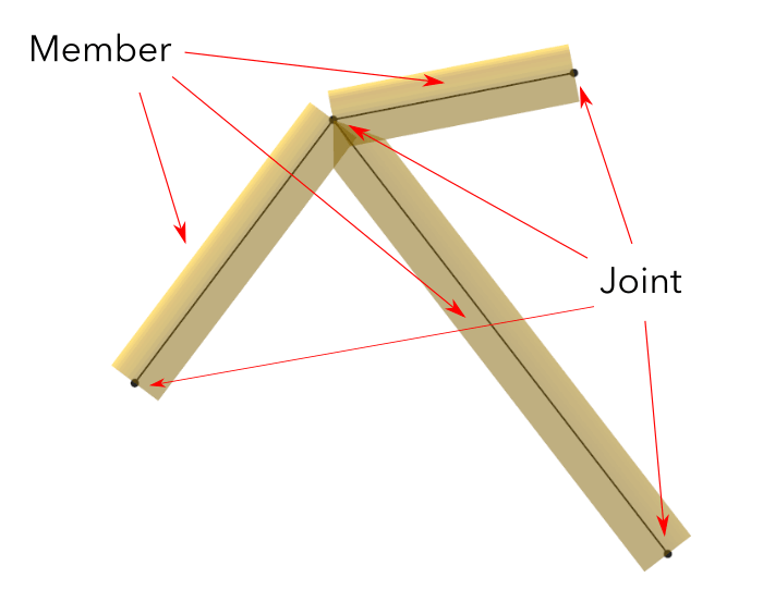
In general, a substructure consists of Members that are defined between Joints. A Member is a cylindrical or rectangular element that connects two Nodes. A Member is oriented along the vector that connects the two Joints, this vector also defines the Members length. A Member can either be defined as rigid or as flexible. When several members are defined between the same joint(s), these members are rigidly connected through the common joints (see Fig. 119).
Fig. 119 Three cylindrical members defined between four joints of a substructure.
Joints are defined via the SUBJOINTS table. A joint is defined by its position and optionally by its orientation. In most cases, it is sufficient to define only the position of the joint, however when imposing constraints along certain degrees of freedom of a joint the joint orientation becomes important. Joints generally dont have a mass, but can be assigned a mass using the ADDMASS_<JntID> keyword.
Fig. 120 Three subjoints and their coordinate system (x-red, y-blue, z-green).
SUBJOINTS
Defines a table that is used to place spatial joints that help define the members of the substructure. Each row of the table defines one joint and has four entries: the first gives the id number of the joint and the other three the Cartesian coordinates of the joint (in m). The origin is the seabed if ISFLOATING is false and the MSL if ISFLOATING is true.
The table is structured as follows:
Listing 48 : The SUBJOINTS table, no orientation defined
By default, the SUBJOINTS are translated and rotated alongside the floater when subjected to initial heave, surge, sway, yaw, pitch, or roll displacements. However, this behavior may be undesirable in certain cases, such as when the SUBJOINTS serve as endpoints for linear springs designed to stabilize the floater (e.g., during a tank test campaign). To address this, you can assign a JntID a negative value. For instance, setting JntID to -1 will globally fix that joint, preventing it from translating or rotating with the initial floater displacements. Despite the negative assignment, the JntID is always treated as a positive value for identification purposes (e.g., in the MOORMEMBERS table). It is important to note that you cannot assign JntID values of -1 and 1 to separate joints simultaneously, as the system treats both as equivalent.
SUBJOINTS (orientation defined by y- and y-axes)
Defines a table that is used to place spatial joints that help define the members of the substructure. Each row of the table defines one joint and has four entries: the first gives the id number of the joint and the other three the Cartesian coordinates of the joint (in m). The origin is the seabed if ISFLOATING is false and the MSL if ISFLOATING is true.
The values X1, Y1, Z1, X2, Y2 and Z2 are optional and can be used to define the local coordinate axes of the joint. X1, Y1 and Z1 are defining the vector of the joints local X-Axis (in global coordinates). X2, Y2 and Z2 define the joints Y-Axis (in global coordinates). The Z-Axis is then constructed to define a right-hand coordinate system. The standard joint orientation is X1, Y1, Z1 = (1,0,0) and X2, Y2, Z2 = (0,1,0). If the user wants to define joint orientations they have to be defined for each joint in the table.
The table is structured as follows:
Listing 49 : The SUBJOINTS table, with orientations defined by x- and y-axes
An alternative way to define the orientation of the substructure joints is to define the orientation of each joint by means of three consecutive Euler rotations around the global coordinate system. The first rotation is performed around the global X-axis, the second rotation around the global Y-axis and the third rotation around the global Z-axis. The last three columns are also optional, if not defined the orientation of each joint is the same as the global coordinate system.
Listing 50 : The SUBJOINTS table, with orientation defined by Euler angles
Defines a table that can be used to apply a global offset to the positions of all SUBJOINTS. Note that the offset is only applied to the joints and not the mass and hydro reference points defined in Linear Potential Flow Modelling.
Defines a table that can be used to apply a global rotation to the positions of all SUBJOINTS (rotation around (0,0,0)). Note that the rotation is only applied to the joints and not the mass and hydro reference points defined in Linear Potential Flow Modelling. This table reads in the rotation angles in degree.
The table is structured as follows:
Listing 52 : The JOINTROTATION table (rotation in °)
JOINTROTATIONXROT YROT ZROT0 0 90
ADDMASS_<JntID>
can be used to add a mass at a joint <JntID>. ADDMASS_<JntID> can be followed by up to 7 numeric values (at least one) to assign mass and rotational inertia properties. For example: ADDMASS_510123456 adds a mass of 10kg at the joint with ID 5. The following numbers assign the rotational inertia in local joint coordinates: Ixx = 1, Iyy = 2, Izz = 3, Ixy = 4, Ixz = 5, Iyz = 6.
can be used to add a constant force, defined in the global coordinate system, to a joint <JntID>. ADDFORCE_<JntID> can be followed by up to 6 numeric values (at least one) to assign forces and moments. For example: ADDFORCE_5123456 applies a force vector of (1,2,3)N and a torque vector of (4,5,6)Nm to joint ID 5. All forces and moments are defined in the global coordinate system.
can be used to add a constant force, defined in the local joint coordinate system, to a joint <JntID>. ADDFORCELOC_<JntID> can be followed by up to 6 numeric values (at least one) to assign forces and moments. For example: ADDFORCELOC_5123456 applies a force vector of (1,2,3)N and a torque vector of (4,5,6)Nm to joint ID 5. All forces and moments are defined in the local joint coordinate system.
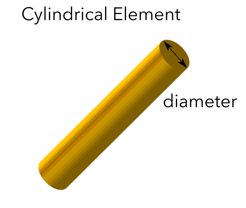
Four different types of element exists that can be used to construct the substructure geometry in the SUBMEMBERS table. Each element definition, identified by a unique Element ID, can be used to generate multiple members. The available element types are: cylindrical flexible elements, cylindrical rigid elements, rectangular flexible elements and rectangular rigid elements.
Fig. 121 A cylindrical element, geometry defined by its end-joints and the diameter.
SUBELEMENTS
Defines a table that defines flexible cylindrical elements that can be used for the substructure definition. Each row represents one (cylindrical) element, which is defined by its structural parameters.
When setting up the substructure, one SUBELEMENT definition can be used for several SUBMEMBERS (see below). Each row has 20 entries. These define the structural parameters of the element.
The entry placement is very similar to the blade and tower structural element table (see Blade, Strut and Tower Structural Data Files). However, there two important differences:
The first entry is used to indicate the ID number of the element (ElemID).
The last (20th) entry is used to indicate the Rayleigh damping of the element.
Defines a table that defines rigid elements that will be used for the substructure definition. Each row represents one (cylindrical) element, which is defined by two attributes: its mass density and its diameter.
When setting up the substructure, one SUBELEMENTRIGID definition can be used for several SUBMEMBERS (see below). An exemplary table is shown below.
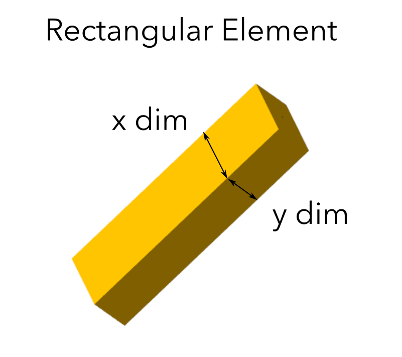
Fig. 122 A rectangular element, geometry defined by its end-joints and its x and y dimension.
SUBELEMENTS_RECT
Defines a table that defines rectangular flexible elements that will be used for the substructure definition. Each row represents one (rectangular) element, which is defined by its structural parameters.
The only difference between the SUBELEMENTS_RECT and the SUBELEMENTS tables is that the element dimensions along its local x-axis (XDIM column 19) and its local y-axis (YDIM column 20) need to be specified, instead of the cylindrical diameter. Thus, two additional values are required and the Rayleigh damping coefficient is shifted to column 22 accordingly. The diameter is in this case only used as a hydrodynamic equivalent diameter for the calculation of Morison forces at the end faces of a member (if a HYDROJOINTCOEFF is defined for one of the members end nodes).
Defines a table that defines rectangular rigid elements that will be used for the substructure definition. Each row represents one (rectangular) element, which is defined by four attributes: its mass density, its dimensions along the local x- and y-axis and an equivalent hydrodynamic diameter which is used to evaluate hydrodynamic forces at the members end faces.
When setting up the substructure, one SUBELEMENTRIGID_RECT definition can be used for several SUBMEMBERS (see below). An exemplary table is shown below.
A multiplication factor that affects the stiffness of the flexible elements defined in SUBELEMENTS.
MASSTUNER
A multiplication factor that affects the mass density of ALL elements defined in SUBELEMENTS.
Assigning Aerodynamic Drag to Substructure Elements
Optionally, the user can assign aerodynamic drag coefficienr in a substructure element table. To do this the aerodynamic drag coefficients are assigned by adding an optional extra column to the substructure element table. The aerodynamic drag is only acting on a substructure member when it is located above the mean sea level (MSL) in an offshore simulation (e.g. poking out of the water). In an onshore simulation the aerodynamic drag value has no effect, instead the HYDROMEMBERCOEFF table is used to assign aerodynamic drag.
The members of the substructure are defined within the SUBMEMBERS table. Each line in the table generated one element that is defined by an element definition, identified by its Element ID and two joints, defined by their Joint ID. In addition the SUBMEMBERS table assigns the member rotation (for rectangular elements) hydrodynamic coefficients, marine growth, flooded area and the discretization for each member.
SUBMEMBERS
Defines a table that contains the members that make up the turbine substructure. A member, with the ID MemID, is defined between two entries of the SUBJOINTS table (Jnt1ID and Jnt2ID) and one entry from an element table (ElmID) (SUBELEMENTS, SUBELEMENTSRIGID, SUBELEMENTS_RECT, SUBELEMENTSRIGID_RECT). The column ElmRot can be used to rotate the member around its principal axis. Rotations are entered in degree.
Additionally, it can have one Morison force coefficients group (HyCoID) defined in the HYDROMEMBERCOEFF table and a marine growth entry (MaGrID) from the MARINEGROWTH table. Also, this table allows the member to be flooded via a flooded cross sectional area entry in [m^2] (FldArea). The member can be subdivided into smaller elements for a more accurate structural and hydrodynamic evaluation. This is done in the MemDisc column; it gives the maximum allowed length of a discrete structural element of the member in [m]. Also, this table has the option to scale the buoyancy forces (IsBuoy) for the individual members (from 0 to 1). It is also possible to use a negative value in the IsBuoy column. In this case the member buoyancy is treated as static, e.g. the MSL is used during buoyancy calculations for this member. Finally, the member can be optionally named for easier recognition in the output tables (Name). The last three optional columns can be used to assign a unique color, specified by its RBG components (Red, Green, Blue), to the member.
When multiple members are connected to the same joint these members are rigidly constrained through this common joint. By using the SUBCONSTRAINTS table it is possible to constrain arbitrary joints, and thereby also the element connected to those joints. The SUBCONSTRAINTS table also allows to fix a joint or to connect a joint with the transition piece, which connects to the turbine structure. The joints can be constrained along any of their degrees of freedom (DoF). Furthermore, it is possible to constrain joints with a spring or damper, instead of a rigid constraint.
SUBCONSTRAINTS
Defines the table that defines the constraints between two joints that are not already connected by members, constraints of joints to the ground or to one TP_INTERFACE_POS transition piece point.
Each row of the table has 12 entries. The first entry defines the constraint ID number (CstID). The next entry define the joint which shall be constrained (JntID). The joint can now be constrained to a second joint, by inserting the corresponding JntID into the JntCon column, to a TP_INTERFACE_POS by inserting its number into the 4th column (TpCon) or to the ground by setting the GrdCon column to 1. A joint can either be constrained to a second joint (JntCon), to the transition piece (TpCon) point or to the ground (GrdCon), so only one of these three columns should be used at the same time.
The sixth entry specifies that the constraint is realized as a non-linear spring-damper element (defined via an the spring ID number). If no spring or damper element is selected the constraint is realized as a stiff connection.
The last 6 entries specify which degrees of freedom are constrained (either stiff or with a spring damper element): the three translational and three rotational degrees of freedom. For these entries 0 is interpreted as unconstrained (free) and 1 is interpreted as constrained. A spring-damper element is always acting along all the constrained degrees of freedom at the same time.
The coordinate system in which the constraints are defined is the coordinate system of JointID1.
An exemplary SUBCONSTRAINTS table is shown below. In this example all joints in the table are connected directly to the transition piece.
Note that at least one joint of the substructure members SUBMEMBERS should be constrained to the transition piece (defined by TP_INTERFACE_POS), to connect the member to the tower bottom of the wind turbine.
Connections to a Second Transition Piece
A joint can be connected to any created transition piece by entering number of the TP_INTERFACE_POS_<X> into the TpCon column.
Connections to the Torquetube
When building a floater for a vertical axis wind turbine (VAWT) the user also has the option to connect a joint to the bottom of a rotating torquetube. This is done by inserting a negative number into the TpCon column. So to connect to the torquetube of the 1st turbine, the user would insert -1 into column TpCon. To connect to the torquetube bottom of the second turbine insert -2.
It is also possible to connect a joint to the top of the torquetube of any turbine, to do this subtract 100 from the value inserted in the TpCon column. As an example: to connect to the torquetube top of the second turbine (located at TP_INTERFACE_POS_2) insert -102 in the TpCon column.
Connections to the Tower Top
Connections to the tower top are realized in a similar way as connections to the torquetube top. By adding 100 into column TpCon. So to connect to the tower top of turbine 1 insert 101 in column TpCon.
TSDA (Translational Spring Damper)
A simple TSDA element can directly be defined between two joints by setting the entry in the Spring column to -1. The spring stiffness is then defined in the DoF_X column, the damping in the DoF_Y column and the rest length \(L_0\) in the column DoF_Z.
Listing 62 : exemplary definition of a TSDA element
In QBlade versions prior to 2.0.7 the constraint degrees of freedom were always defined in the coordinate system of the object to which Jnt1ID was constrained, e.g. Joint2ID, the transition piece or the ground. From QBlade 2.0.7 on the coordinate system for the constraint is now that of Jnt1ID.
The transition piece is the reference position in the substructure definition that defines the interface between the turbine definition and the substructure. It is possible to connect the substructure either to the tower bottom, to the torquetube bottom or directly to the rotor nacelle assembly (RNA) of a turbine definition. If the main structural input file contains a TWRFILE the transition piece of the substructure (TP_INTERFACE_POS) is automatically connected to the tower bottom. If the substructure contains no TWRFILE keyword the transition piece is connected to the rotor nacelle assembly (RNA). Through the SUBCONSTRAINTS table joints (and their connected members) can be connected to the transition piece.
TP_INTERFACE_POS_<X>
Defines the (x,y,z) coordinates (in m) of the position of the transition piece location of the substructure. It is defined as the point where the substructure is connected to the tower base of the wind turbine.
For floating substructures it is defined in (x,y,z) [m] from the MSL = (0,0,0).
For bottom fixed substructures, it is defined from the seabed.
Note that the inertia and hydrodynamic reference points (REF_COG_POS and REF_HYDRO_POS) are always automatically constrained to this point (see Linear Potential Flow Modelling). There can be several transition piece points. Further points are then defined by adding additional keywords where an underscore and a number is added to the keyword (e.g. TP_INTERFACE_POS_2). This allows the user to define additional inertia and hydrodynamic reference points (see Linear Potential Flow Modelling). If a multi-rotor wind turbine is simulated the TP_INTERFACE_POS_1 would automatically connect to the tower bottom of turbine 1, TP_INTERFACE_POS_2 would automatically connect to the tower bottom of turbine 2 and so on.All transition piece points can be constrained to a joint of the substructure in the SUBCONSTRAINTS table.
The structure of the table is:
Note: for the 1st TP_INTERFACE_POS_<X> the numbering _1 can be omitted, so TP1 can be defined by the keyword TP_INTERFACE_POS. This is also true for the definitions of all following reference points.
TP_ORIENTATION_<X> (orientation defined by x- and y -axes)
Defines the orientation of the tower base or RNA coordinate system which is connected to the TP_INTERFACE_POS_<X> by defining its \(X_t\)- and \(Y_t\)-Axis in the global coordinate system. The first row defines the X-axis (\(X_{tp}\)) orientation and the second row defines the Y-axis (\(Y_{tp}\)) orientation of the transition piece coordinate system.
If TP_ORIENTATION_<X> is not specified the default values are \(X_{tp}=(1,0,0)\) and \(Y_{tp}=(0,1,0)\), so the tower base coordinate system is aligned with the global coordinate system. The \(Z_t\)-Axis is evaluated from the cross-product of \(X_t\) and \(Y_t\).
TP_ORIENTATION_<X> (orientation defined by Euler angles)
An alternative way of defining the orientation of the tower base or RNA is to specify the orientation by means of three Euler angles. Starting from the global coordinate system three consecutive Euler rotations are performed, first around the global X, second around the global Y and third around the global Z axis.
In the context of floating offshore structures, the neutral point is defined as the origin (0,0,0) in the local floater coordinate system. The floater’s dynamic behavior, including translations and rotations, is typically referenced to this point. During the ramp-up phase of a simulation, the floater remains fixed at its neutral point to allow the mooring lines to settle into their equilibrium shape. By default, the neutral point is rigidly constrained to TP_INTERFACE_POS_1, ensuring that TP_INTERFACE_POS_1 remains fixed during this initial phase. If the user wishes to override this default constraint and constrain the neutral point (NP) to a different joint, this can be done using the NPSUBJOINT keyword.
NPSUBJOINT
This keyword can be used to constrain the neutral point to an arbitrary substructure joint. This overrides the default setting where the neutral point is constrained to TP_INTERFACE_POS_1.
Listing 66 : The neutral point is constrained to SUBJOINT 12
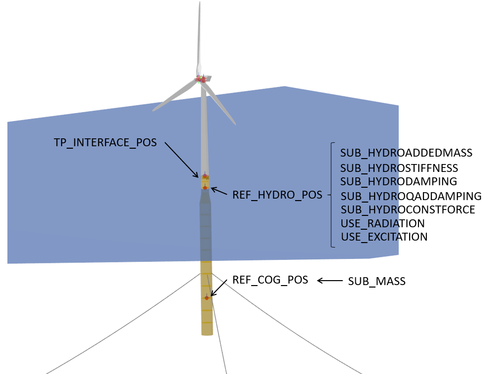
Fig. 124 Main reference points for the substructure. The inertia reference point REF_COG_POS and the hydrodynamic reference point REF_HYDRO_POS are constrained to the transition piece point TP_INTERFACE_POS.
For each transition piece multiple reference position exist, which are rigidly constrained with the transition piece. These reference points can be used to assign lumped masses, lumped hydrodynamic forces (such as linear stiffness or damping) or lumped hydrodynamic added mass. The REF_HYDRO_POS_<X> reference point also acts as the position at which the forces from linear potential flow data are applied to the substructure (see Linear Potential Flow Modelling).
REF_COG_POS_<X>
defines the (x,y,z) position (in m) of a inertia point of the system (i.e. the center of gravity). It is in this position that the SUB_MASS matrix is evaluated. This point is automatically constrained to the transition piece, defined by TP_INTERFACE_POS. It has the following format:
defines a complete 6 by 6 mass and rotational inertia matrix that is placed in the location defined by the REF_COG_POS_<X> keyword. The units are kg for the mass and kg m^2 for the inertia. An example of this matrix is shown below:
defines the (x,y,z) position (in m) of a hydrodynamic evaluation point of the system (i.e. where the lumped hydrodynamic forces are applied). It is in this position that the hydrodynamic matrices (e.g. SUB_HYDROSTIFFNESS_<X>, SUB_HYDRODAMPING_<X>, SUB_HYDROADDEDMASS_<X>, etc.) and the radiation and excitation forces are applied. This point is directly constrained to the TP_INTERFACE_POS_<X> point, so no additional constraints are necessary to attach this point to the substructure. It has the following format:
defines a complete 6 by 6 stiffness matrix that is evaluated in the location defined by the REF_HYDRO_POS_<X> keyword. The units are N/m, N/rad, Nm/m, Nm/rad, depending on the entry. The general form of this matrix is shown below:
defines a complete 6 by 6 damping matrix that is evaluated in the location defined by the REF_HYDRO_POS_<X> keyword. The units are N/(m/s), N/(rad/s), Nm/(m/s) or Nm/(rad/s), depending on the entry. This matrix has the same form as the SUB_HYDROSTIFFNESS_<X> matrix.
SUB_HYDROQUADDAMPING_<X>
defines a complete 6 by 6 quadratic damping matrix that is evaluated in the location defined by the REF_HYDRO_POS_<X> keyword. The units are N/(m/s)^2, N/(rad/s)^2, Nm/(m/s)^2, Nm/(rad/s)^2, depending on the entry. This matrix has the same form as the SUB_HYDROSTIFFNESS_<X> matrix.
SUB_HYDROADDEDMASS_<X>
defines a complete 6 by 6 added mass matrix that is evaluated in the location defined by the REF_HYDRO_POS_<X> keyword. The units are kg. This matrix has the same form as the SUB_HYDROSTIFFNESS_<X> matrix.
SUB_HYDROCONSTFORCE_<X>
applies a constant force (and/or torque) to the REF_HYDRO_POS_<X> point. It can be used to e.g. model the constant buoyancy force acting on the floater in its equilibrium position. The units are N or Nm, depending on the entry.
applies a constant force in the global z-direction to the REF_HYDRO_POS_<X> point that is calculated based on the displaced water volume given by the user. It can be used to e.g. model the constant buoyancy force acting on the floater in its equilibrium position in a simple way without evaluating the force directly. This force is added to the SUB_CONSTFORCE_<X> entries, but can be used without specifying SUB_CONSTFORCE_<X>.
Fig. 125 Mooring lines connected to a floating wind turbine for ground fixing.
The connection to the ground is handled differently for floating and fixed-bottom substructures. For floating substructures, the anchoring is done via the mooring lines defined with the MOORELEMENTS and
MOORMEMBERS keywords. These keywords can also be used to define flexible cable elements of the substructure. For bottom-fixed substructures, the connection to the ground is defined in the SUBCONSTRAINTS table.
It can be either a rigid connection or a connection via a system of non-linear springs and dampers. These latter elements are defined with the keywords NLSPRINGDAMPERS and optionally SPRINGDAMPK.
MOORELEMENTS
is a table that contains the structural parameters of the flexible cable elements of the substructure such as mooring lines. Each row defines one set of parameters and has 6 values. These are the mooring element ID number, the mass per length [kg/m], bending stiffness around y or x in [Nm^2], the axial stiffness in [N], a structural (longitudinal) damping coefficient and a hydrodynamic diameter in [m], which are used during buoyancy and Morison force evaluations.
Optionally, a nonlinear axial stiffness for a MOORELEMENT may be defined by a nonlinear data table (see Nonlinear Data Tables). In this case, the data table identifier, preceded by a hashtag (#) replaces the EA value of the MOORELEMENTS table.
In some cases, if the alpha damping coefficient of a mooring line (or cable) element is too large, a simulation can become unstable. Therefore, by default the damping coefficient of the mooring lines is not applied. If the user wishes to activate the axial damping of mooring lines and guy cables, the keyword CABDAMP must be set to true.
Listing 75 : Activating axial cable damping for all MOORELEMENTS be setting the keyword CABDAMP
true CABDAMP
MOORMEMBERS
is a table that contains the information of the cable members (such as the mooring lines). Each row defines one cable member and has 10 entries. The first entry is the ID number of the cable member. The next two entries are the connection points of the cable member. There are several ways of defining the connection points. These are:
With the keyword JNT_<ID>, where <ID> represents the ID of the joint. This way, the cable is connected directly to a existing joint.
With the keyword FLT_<XPos>_<YPos>_<ZPos>, where <XPos>_<YPos>_<ZPos> represent the global (x,y,z) coordinates of the connection point (in m). Here, QBlade creates a constraint between this point and the floater to attach the cable.
With the keyword GRD_<XPos>_<YPos>, where <XPos>_<YPos> represent the global (x,y) (in m) coordinates of an anchor point which is located at the z-position of the seabed.
With the keyword BLD_<X>_<Y>, blade X at the normalized curved length position Y.
With the keyword STR_<X>_<Y>_<Z>, connects to strut Y of blade X at the normalized curved length position Z.
With the keyword TWR_<X>, connects to the tower at the normalized position X.
With the keyword TRQ_<X>, connects to the torquetube, at the normalized position X.
The fourth entry is the length of the cable (in m). The fifth entry is the ID number of the cable element defined in MOORELEMENTS. The sixth entry is the ID number of the hydrodynamic coefficient group defined in HYDROMEMBERCOEFF.
The seventh entry specifies if the cable is buoyant (= 1) or not (= 0). The eighth entry specifies the ID number of the marine growth element used for this cable (see MARINEGROWTH). The ninth entry is the number of discretization nodes used
to discretize the cable and the tenth entry is the name of the cable element.
It is also possible to assign offsets to mooring line connections when connecting to blades, struts, the tower, or the torquetube. These offsets are defined similarly to the offsets for cable connections; see Applying Offsets to cables.
The offsets are specified in the local coordinate system of the connected body using x, y, and z coordinates, appended after the length position.
For example, BLD_1_0.5_0_1_1 applies an offset of 1m in the local y and z directions of the blade.
MOORCONSTRAINTS
By default, only the position of the mooring line end nodes is constrained in the MOORMEMBERS table. The MOORCONSTRAINTS table can optionally be used to also constrain the orientation of a mooring line. This table requires seven columns, which define two unit directional vectors for the start and end nodes of the mooring line. These directional vectors are specified in one of the following coordinate systems:
Global Coordinate System (GRD): For connections to the ground.
Joint Coordinate System (JNT): If connected to a joint.
Floater Coordinate System (FLT): If connected to the floater.
The columns required in the MOORCONSTRAINTS table are:
ID: The ID of the mooring line, as defined in the MOORMEMBERS table.
C1_X: The X-component of the directional (unit) vector at the start node.
C1_Y: The Y-component of the directional (unit) vector at the start node.
C1_Z: The Z-component of the directional (unit) vector at the start node.
C2_X: The X-component of the directional (unit) vector at the end node.
C2_Y: The Y-component of the directional (unit) vector at the end node.
C2_Z: The Z-component of the directional (unit) vector at the end node.
is a table that allows to add buoyancy loads or additional weight to a cable member defined in the MOORMEMBERS table. The first column is the cable member ID, the second column the starting position of the load, the third column is the end position of the load and the fourth column the load itself, defined in [N/m]. The loads only act along the global Z-Axis. A positive load is pointing upwards and a negative load is pointing downwards.
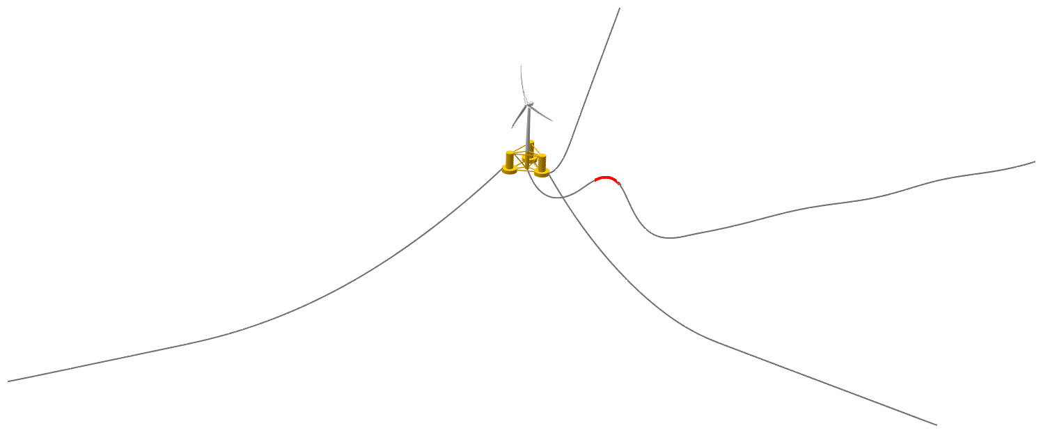
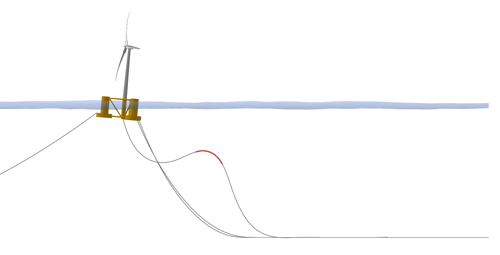
Fig. 126 A buoyancy load acting on a power cable.
is a table that defines one or more non-linear spring-damper systems for connecting the substructure to the ground, or for the interconnection of two joints in the constraints table. A usual application would be to model the soil dynamics using nonlinear (p-y curves) springs. Another application would be to define compliant connections between substructure members or joints. Furthermore, in the SUBCONSTRAINTS table the nonlinear springs, or dampers may be assigned to constrain any or all degrees of freedom of choice.
Each row in the NLSPRINGDAMPERS table represents a spring-damper system and has 2N + 2 entries, where N is the number of points on the definition table of the non-linear spring/damper. The first entry represents the ID number of the system (to be used in the SUBCONSTRAINTS table). The second entry defines the type of connection that is being modeled. There are two options: ‘spring’ and ‘damp’. This affects the way the coefficients in the following entries are interpreted.
If ‘spring’ is selected, then QBlade expects the definition table to consists of displacement or rotation (in m or rad) and stiffness (in N/m or Nm/rad) entries.
If ‘damp’ is selected, then QBlade expects the definition table to consist of velocity (in m/s or rad/s) and damping (in N(m/s) or Nm/(rad/s)) entries.
When a spring or damper is used to constrain two joints its nonlinear definition always acts as a rotational spring or damper along the rotational DOF’s and as a translational spring or damper along the translational DOF’s. Thus, usually a spring is either defined as a rotational spring and then assigned to constrain rotational DOF’s or as a translational spring to constrain translational DOF’s.
The following 2N entries represent the additional lookup table entries for the non-linear spring/damper system. The order is \(x_1/v_1\), \(K/D(x_1/v_1)\); \(x_2/v_2\), \(K/D(x_2/v_2)\) and so on. Each spring/damper force displacement relationship is assumed to go through the origin at \(x_0/v_0 = 0\) and \(K/D(x_0/v_0) = 0\).
NLSPRINGDAMPERSElemID Type Coefficient & Displacement/Velocity Sets (for NL springs, dampers)1 spring 1.000 1.160E+06 2.000 2.21E+062 spring 1.000 9.000E+06 2.000 1.20E+073 spring 1.000 2.090E+07 2.000 2.10E+074 spring 1.000 3.560E+07 2.000 3.30E+07
Optionally, the force/displacement or force/velocity relationship can also be specified though a Nonlinear Data Tables. In this case, the data table ID, preceded by a hashtag (#), replaces the 2N lookup table entries in the NLSPRINGDAMPERS table.
Listing 80 : The NLSPRINGDAMPERS table, using data from a NLDATA table
NLSPRINGDAMPERSElemID Type Coefficient & Displacement/Velocity Sets (for NL springs, dampers)1 spring #NLDATA12 spring #NLDATA23 spring #NLDATA34 spring #NLDATA4
SPRINGDAMPK
is an optional proportionality constant to add a damping value to the spring elements. If this keyword is used, then all of the spring elements defined in NLSPRINGDAMPERS are treated as spring-damping systems. The additional damping coefficients are calculated using the following approach: \(D_i\) = SPRINGDAMPK\(\cdot K_i\). This keyword does not affect the ‘damp’ elements defined in NLSPRINGDAMPERS.
Changes to in NLSPRINGDAMPERS QBlade 2.0.7
From QBlade 2.0.7, the NLSPINGDAMPERS table has been slightly modified. In Previous versions the coefficient for \(x=0\) was specified by the user in column 3 of the table. In the new table format column 3 is now removed and the force/dsplacement, or force/velocity, relationship is always going through the origin at \(x_0/v_0 = 0\) and \(K/D(x_0/v_0) = 0\). This implies that in order to continue to use a NLSPINGDAMPERS table from a QBlade version prior 2.0.7 the 3rd column has to be removed. The old table format is shown below for reference:
Listing 81 : The old NLSPRINGDAMPERS table, not working anymore!!
NLSPRINGDAMPERSElemID Type Coefficient (for x = 0) Coefficient & Displacement/Velocity Sets (for NL springs, dampers)1 spring 0.000E+00 1.000 1.160E+062 spring 0.000E+00 1.000 9.000E+063 spring 0.000E+00 1.000 2.090E+074 spring 0.000E+00 1.000 3.560E+07
P-y curves are a widely used method for modeling soil resistance as a function of pile displacement in soil-structure interaction. In QBlade, these curves can be defined using the NLSPRINGDAMPERS table, which allows direct input of force-displacement pairs to capture the nonlinear behavior of soil.
Identify Interaction Joints:
Determine the substructure joints where soil-structure interaction will be modeled, typically those located below the seabed.
Define P-Y Curves in :code:`NLSPRINGDAMPERS`:
Use the NLSPRINGDAMPERS table to directly input the force-displacement pairs for the p-y curve. For each nonlinear spring element:
Assign an element ID (ElemID) and specify the type (spring for p-y curves).
Provide the displacement and corresponding force pairs.
Example:
Listing 82 NLSPRINGDAMPERS Table with P-Y Curve Data
NLSPRINGDAMPERSElemID Type Displacement & Force Pairs1 spring 0.001 10000 0.005 20000 0.01 30000 1.0 30000
At a displacement of \(0.001\) m, the soil provides \(10000\) N of resistance.
At \(0.005\) m, the resistance increases to \(20000\) N.
At \(0.01\) m, the resistance reaches \(30000\) N.
For displacements exceeding \(0.01\) m, the resistance plateaus at \(30000\) N, indicated by the final force-displacement pair. A plateau, indicating ultimate resistance is automatically detected when the last two force/displacement pairs have equa force values.
Assign Nonlinear Springs inSUBCONSTRAINTS:
Link the nonlinear spring elements to constrain specific degrees of freedom (DOFs) at the interaction points. Assign the spring to act along translational DOFs to represent lateral soil resistance.
Reference External Data Tables (Optional):
For extensive or separately stored p-y data, use a predefined nonlinear data table (NLDATA) instead of directly entering displacement-force pairs. Replace the force-displacement entries in the NLSPRINGDAMPERS table with the reference ID:
Listing 83 NLSPRINGDAMPERS Table with Referenced Data
NLSPRINGDAMPERSElemID Type Displacement & Force Pairs1 spring #NLDATA1
Ensure that NLDATA1 contains the corresponding p-y curve data.
Set Proportional Damping (Optional):
Add damping to the nonlinear springs using the SPRINGDAMPK keyword:
0.05 SPRINGDAMPK
This applies proportional damping to the force-displacement relationship, where damping coefficients are calculated as \(D_i = \mathrm{SPRINGDAMPK} \cdot K_i\).
Caution: Correctly Integrating Force Values
Typically, the resistance force in p-y curves is expressed in terms of force per unit pile length (\(\frac{N}{m}\)). Since the spring elements in QBlade act on the nodes of a member, the force values defined in the NLSPRINGDAMPERS table must be integrated according to the length of the associated member.
In QBlade, nonlinear springs can model elastic perfectly-plastic behavior, meaning the spring response is fully recoverable until the ultimate soil resistance is reached. The ultimate soil resistance is reached when the user defined p-y- curve reaches a plateau (see NLSPRINGDAMPERS Table with P-Y Curve Data). As the lateral displacement increases and the p–y curve approaches its plateau (representing the soil’s ultimate resistance), the behavior transitions to plastic deformation, where any additional displacement results in permanent deformation. To capture this behavior, an elastic perfectly plastic hysteresis model is implemented (see Fig. 127), ensuring that the model accurately represents the transition from elastic (recoverable) to plastic (permanent) behavior.
In QBlade, nonlinear springs can model elastic perfectly-plastic behavior, ensuring an accurate representation of soil response. The soil resistance increases elastically until the ultimate soil resistance is reached, at which point it plateaus and transitions to plastic deformation. This is defined in the p-y curve by the plateau in the force-displacement pairs (see NLSPRINGDAMPERS Table with P-Y Curve Data).
To model this behavior, QBlade uses an elastic perfectly-plastic hysteresis model (see Fig. 127). This ensures that the transition from elastic (recoverable) to plastic (permanent) behavior is captured accurately.
is a table that defines a nonlinear data distribution. The type as which the data is interpreted, depends on where the data table is used. Currently, nonlinear data tables can be used to define nonlinear stress/strain relationships for the axial (EA) stiffness of mooring lines (see Mooring Elements) or to define the force/displacement relationships of spring (or damper) elements (see Nonlinear Spring and Damper Constraints).
Each nonlinear data table needs a unique identifier, such as NLDATA1, NLDATA2, NLDATA3, up to NLDATA100. The first column in each data table represents the x-value (such as displacement, velocity or strain) and the second column represents the y-axis (such as force or stress. A nonlinear data table is assumed to always go through the origin at x=0 and y=0 and it is not requires to input the 0,0 entry into the table. Other values should be input is ascending order of x.
Two options are available in QBlade to model the hydrodynamic forces acting on an offshore substructure: The Morison equation and the linear potential flow theory.
When modeling the hydrodynamics using the Morison equation the user can distribute hydrodynamic coefficients that act in the normal direction of a substructure member. Furthermore, coefficients can be added to substructure joints so that the Morison equation is applied to the end faces of members. Thus, when modeling the hydrodynamics using the Morison equation the hydrodynamic forces are distributed over the substructure model.
The second option is to model the hydrodynamic forces using a linear potential flow theory generated database. At present, QBlade can interpret hydrodynamic input data in the WAMIT and NEMOH formats. When modeling hydrodynamics with potential flow theory the lumped hydrodynamic forces are always applied at the hydrodynamic reference point (REF_HYDRO_POS_<X>). So, in most cases, a substructure modeled with potential flow theory should be modeled using rigid elements.
QBlade allows the user to combine elements from the Linear Potential Flow Theory and Morison Equation hydrodynamic models freely. The user should be careful when setting up the substructure in QBlade so that the model remains consistent.
A typical mix between the Morison equation and potential flow theory is to have all hydrodynamic forces be evaluated by a linear potential flow database and use the Morison equation to compute the hydrodynamic drag force, which is missing from the potential flow theory due to its assumption of inviscid flow.
Morison Element Behavior in On- and Offshore Simulations
Morison strip theory can be used to assign drag, added mass and damping coefficients to elements of the substructure. Typically this is used in an offshore simulation where the Morison forces are applied to the submerged members based on the water density. In case Morison coefficients are applied to a substructure that is used in an onshore simulation all members are treated as submerged and the air density values is used to evaluate the Morison forces. See also Marine Hydrokinetic Turbines.
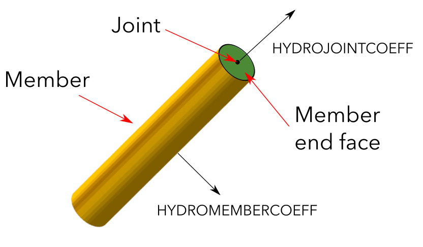
Hydrodynamic coefficients can be assigned to substructure members and joints. Hydrodynamic member coefficients (HYDROMEMBERCOEFF) act in the direction normal to the center-line of the substructure member. Hydrodynamic joint coefficients act in the direction normal to the end face of a member (see Fig. 128).
Fig. 128 Hydrodynamic coefficients acting on a substructure member.
HYDROMEMBERCOEFF
defines a table that contains the hydrodynamic normal coefficients that are used for the cylindrical members of the substructure. Each row contains one group of coefficients that can be used by one or more cylindrical members. The table contains a minimum of five entries, with an optional sixth entry. These are the ID number of the group, the normal drag coefficient, the normal added mass coefficient, the normal dynamic pressure coefficient, a flag that enables the MacCamy-Fuchs correction (MCFC) and an optional entry for an axial drag coefficient CdAx. The last two columns are also optional, and allow to specify a cut off frequency and blend factor alpha to apply a high pass filter to be applied to the viscous drag forces, see High-Pass Filtered Morison Drag.
For cylindrical members, the reference area used for the evaluation of drag forces is the projected member surface area \(A = d \, l\), where \(d\) is the member diameter and \(l\) is the (submerged) member length.
The reference volume used for the evaluation of added mass and Froude–Krylov forces is the member volume \(V = \frac{d^2}{4} \, \pi \, l\).
HYDROMEMBERCOEFF_RECT
defines a table that contains the hydrodynamic normal coefficients that are used for the rectangular members of the substructure. Each row contains one group of coefficients that can be used by one or more rectangular members. The table contains eight entries. These are the ID number of the group, the normal drag coefficient along the members local x-axis, the normal added mass coefficient along the members local x-axis, the normal dynamic pressure coefficient along the members local x-axis, the normal drag coefficient along the members local y-axis, the normal added mass coefficient along the members local y-axis, the normal dynamic pressure coefficient along the members local y-axis and a flag that enables the MacCamy-Fuchs correction (MCFC) and an optional entry for an axial drag coefficient CdAx. The last two columns are also optional, and allow to specify a cut off frequency and blend factor alpha to apply a high pass filter to be applied to the viscous drag forces, see High-Pass Filtered Morison Drag.
For rectangular members, the reference area used for the evaluation of drag forces is the surface area \(A = 2 \, d_{xdim} \, l\) and \(A = 2 \, d_{ydim} \, l\), where \(d_{xdim}\) and \(d_{ydim}\) are the side lengths of the member faces along the members local \(x\) and \(y\) axes and \(l\) is the (submerged) member length. The area is multiplied by a factor of \(2\) to account for both opposing faces of the member. This means CdNx is used in combination with the area calculated with \(d_{ydim}\) and CdNy is used in combination with the area calculated with \(d_{xdim}\).
The reference volume used for the evaluation of added mass forces is calculated as the area of an equivalent circle, obtained from the side length of the member face, multiplied by the submerged member length: \(V_x = \frac{d_{xdim}^2}{4} \, \pi \, l\), and \(V_y = \frac{d_{ydim}^2}{4} \, \pi \, l\), where \(d_{xdim}\) and \(d_{ydim}\) are the side lengths of the member faces. This means CaNx is used in combination with the volume calculated with \(d_{ydim}\) and CaNy is used in combination with the volume calculated with \(d_{xdim}\).
The reference volume used for the evaluation of Froude–Krylov forces is based on the cross-sectional member area and the submerged member length: \(V = d_{xdim} \, d_{ydim} \, l\).
FOILMEMBERCOEFF
This table allows the user to assign lift and drag coefficients of a 360° polar to a substructure member. The aero- or hydrodynamic forces are evaluated based on the current angle of attack experienced by the member. The chord used for force evaluation is the DIAMETER specified for the underlying SUBELEMENT, see Fig. 129.
Fig. 129 A substructure member with an airfoil and polar assigned through the FOILMEMBERCOEFF table.
The visualized chord is equal to the SUBELEMENT diameter.
Below is an exemplary FOILMEMBERCOEFF table. The first column defines the coefficient ID, the second column specifies the airfoil, and the third column lists the associated 360° polar. The last two columns define the pitch axis of the airfoil and whether the airfoil is inverted. Optionally, the user may assign added mass (Ca) and dynamic pressure (Cp) coefficients in columns 6 and 7 of the data table. When an airfoil is assigned to a substructure member, for the purpose of buoyancy calculations, the scaled cross-sectional area of the airfoil is used. The ADVANCEDBUOYANCY feature cannot be used for foiled members.
When aerodynamic forces are evaluated for a foiled member, an iteration for the bound circulation is carried out, similar to the iteration for the bound circulation of a rotor blade when simulating with the Lifting Line Free Vortex Wake method. The convergence criterion epsilon and the relaxation factor can be specified in the substructure file. If not explicitly set, default values are used:
Relaxation Factor: 0.015
Epsilon (Convergence Criterion): 0.005
The Lifting Line at the member position is updated with the circulation calculated at every timestep, and the induction field caused by the Lifting Line influences neighboring elements.
The user can also output the angle of attack, aero- or hydrodynamic force, and moment evaluated at this member by setting AER_OUT to true in the structural input file. See Loading Data and Sensor Locations.
is a table that defines hydrodynamic axial coefficients that can be placed at specific joints (defined by their ID number) of the substructure that are located at the ends of cylindrical members. QBlade assumes a spherical end of the element when calculating the hydrodynamic axial Morison forces (e.g. \(F_a^{ax} = \frac{d^3}{12} \, \pi \, C_a^{ax}\)). The table contains the axial drag, added mass and dynamic pressure axial coefficients and is structured as shown below. The hydrodynamic reference volume for a member end face is assumed to be a semi-spheroid with the member diameter (the equivalent diameter for rectangular members). If two substructure members are connected to the same node the member face reference areas and reference volumes are subtracted from another so that just the area and reference volumes that is exposed to the fluid is considered when evaluating the Morison forces.
The reference area for member end drag forces is evaluated based on the member diameter as \(A = \frac{d^2}{4} \, \pi\). For rectangular members, this formula uses the hydrodynamic diameter \(d\) defined in the element table.
The reference volume for added mass and Froude-Krylov forces is evaluated as the volume of a semisphere, using the hydrodynamic member diameter: \(V = \frac{dia^3}{12} \, \pi\).
In addition to the basic functionalities of the HYDROJOINTCOEFF table additional entries in the table can activate a more advanced modeling of member end Morison forces, to improve the prediction of low frequency responses of floating structures. Two advanced modeling techniques (see Wang et al. 1 and Behrens de Luna et al. 2), named One-Sided Morison Drag and High-Pass Filtered Morison Drag can be activated by optionally populating additional columns in the HYDROJOINTCOEFF table. The OSD, f_cutOff and alpha columns are all optional, and can be omitted if these modeling features are not needed.
WAVEKINEVAL_MOR
is an optional flag that controls how the local wave kinematics are used to calculate the Morison forces (see Modeling Considerations for Morison Elements).
The available options are:
0: local evaluation of wave kinematics (this is the default value if not specified)
1: evaluation at the fixed, undisplaced/unrotated initial reference position
2: evaluation at a lagged position (controlled by WAVEKINTAU).
WAVEKINTAU
is an optional time constant for the first order low-pass filter used to determine lagged position of the Morison/Potential Flow elements (when WAVEKINEVAL_MOR or WAVEKINEVAL_POT is set to 2). The default value is 30s.
The High-Pass Filtered Morison Drag modification is another method to improve, or fine-tune the low-frequency response of a floating structure. To optimize the simulation of freely floating structures in irregular waves, QBlade incorporates an optional high-pass velocity filter for evaluation of the axial drag force on heave plates. This model allows to implement varying drag force across different wave frequency bands. This method uses a first-order high pass filter, which is applied to the relative normal velocity at a members end-face. After Wang et al. 1, the filtered normal velocity (\(\tilde{v}_{i}\)) in discrete time is evaluated as:
\(\tilde{v}_{i} = C \cdot \tilde{v}_{i-1} + C \cdot (v_{i} - v_{i-1})\),
with
\(C = exp(-2\pi f_c \Delta t)\).
The applied filtered drag force \(F_{D,f}\) is then evaluated as:
\(F_{D,f}=\alpha F_D + (1-\alpha) \tilde{F}_D\),
where \(\alpha\) is a scaling factor between 0 and 1, \(\tilde{F}_D\) is the drag force evaluated with the filtered normal velocity \(\tilde{v}_i\) and \(F_D\) the drag force evaluated with the unfiltered normal velocity \(v_i\).
An application of this filtered drag evaluation can be found in the works of Wang et al. 1 and Behrens de Luna et al. 2.
The One Sided Morison Drag method modifies the (axial) drag model used in QBlade by applying the axial drag force solely when the flow normal to the surface is in the direction of the end faces normal vector (\(v \cdot n > 0\)), representing a state of flow separation. This modification is suggested because the potential-flow model already includes the increased stagnation pressure when the flow is the opposite direction of the end face normal vector. This modification more accurately reflects the physical conditions where viscous effects cause a pressure reduction on the flow-facing side, which diverges from the ideal pressure recovery assumed in potential-flow models. This modification modifies the evaluation of the end face drag force in the following way:
\(F_D = \frac{1}{2} C_{d_A} \left| v \cdot n \right| \max(v \cdot n, 0)\)
The one-sided Morison drag evaluation is activated by setting the sixth column of the HYDROJOINTCOEFF table to 1. Setting this column to 0 deactivates this correction:
QBlade supports any number of linear potential flow bodies as part of a substructure definition, where each potential flow body is related to a transition piece TP_INTERFACE_POS_<X>. In order to include multiple bodies, each body has to have its own set of keywords. With the exception of the first body, additional bodies are defined by adding an underscore and a number after the keyword. So, for example, if a substructure has two bodies that use the linear potential flow theory, the second body would be defined by adding a second transition piece point TP_INTERFACE_POS_2 with its corresponding hydrodynamic reference point REF_HYDRO_POS_2, the inertia point REF_COG_POS_2, a mass matrix denoted as SUB_MASS_2 and so on (see the section: Lumped Mass, Inertia and Hydrodynamic Forces).
The keywords that are used to read in the linear potential flow databases for radiation, excitation, difference and sum frequency loads, or hydrodynamic stiffness are detailed below:
defines the position at which the potential flow loads (hydro stiffness, radiation, excitation, sum frequency and difference frequency) are applied. This is also the position at which wave elevations, positions are accelerations are obtained. As detailed in the section Lumped Mass, Inertia and Hydrodynamic Forces, this reference position is automatically constrained with the transition piece`:code:TP_INTERFACE_<X>.
points to the file (.hst) in which the hydrodynamic stiffness matrix is stored from a WAMIT calculation. If this keyword is used then the hydrodynamic stiffness matrix SUB_HYDROSTIFFNESS_<X> is populated with data from the file, overwriting any user-defined stiffness matrix.
POT_RAD_FILE_<X>
points to the file (.1) file in which the radiation coefficients from a WAMIT calculation for the linear potential flow model are located. The file ending must be included. This determines the format of the file. QBlade currently supports radiation files in the WAMIT, NEMOH and BEMUse formats.
POT_EXC_FILE_<X>
points to the file (.3 file) in which the excitation coefficients from a WAMIT calculation for the linear potential flow model are located. The file ending must be included. This determines the format of the file. QBlade currently supports excitation files in the WAMIT, NEMOH and BEMUse formats.
POT_DIFF_FILE_<X>
points to the file (.12d file) in which the second-order difference-frequency wave force coefficients from a WAMIT calculation are located. The file ending must be included. This determines the format of the file. QBlade currently supports difference-frequency files only in the WAMIT format.
POT_SUM_FILE_<X>
points to the file (.12s file) in which the second-order sum-frequency wave force coefficients from a WAMIT calculation are located. The file ending must be included. This determines the format of the file. QBlade currently supports sum-frequency files only in the WAMIT format.
DIFF_CUTOFF_L_<X>
Specifies the low cut-off frequency for the difference QTFs. Intended to speed up the QTF evaluations.
DIFF_CUTOFF_H_<X>
Specifies the high cut-off frequency for the difference QTFs. Intended to speed up the QTF evaluations.
DIFF_INACTIVE_DOF_<X>
this keyword can be used to define a list of DOFs for which the difference QTF will not be evaluated. Intended to speed up the QTF evaluations.
Listing 91 : The DIFF_INACTIVE_DOF keyword to deactivate the DOFs 1 and 4 from the difference QTF evaluation
1 4 DIFF_INACTIVE_DOF
SUM_CUTOFF_L_<X>
Specifies the low cut-off frequency for the sum QTFs. Intended to speed up the QTF evaluations.
SUM_CUTOFF_H_<X>
Specifies the high cut-off frequency for the sum QTFs. Intended to speed up the QTF evaluations.
SUM_INACTIVE_DOF_<X>
this keyword can be used to define a list of DOFs for which the sum QTF will not be evaluated. Intended to speed up the QTF evaluations.
Listing 92 : The SUM_INACTIVE_DOF keyword to deactivate the DOFs 1 and 4 from the sum QTF evaluation
Fig. 130 NBODY=3, 6 DOF’s are assigned to each of the three cylinders.
QBlade includes the capability to include multiple bodies (NBODY>1 feature of WAMIT) that interact hydrodynamically and mechanically. Each body can oscillate independently with up to six degrees of freedom. This extension increases the maximum number of degrees of freedom from 6 for a single body to 6N for N bodies.
POT_NBODY_<X>
specifies the number of hydrodynamic bodies. Each body is associated with 6 DOF’s. By default, NBODY is equal to 1. To use NBODY>1, the potential flow files must contain the data for the additional DOF. If NBODY=3, then the data for 18 DOF’s is required.
Listing 93 : The POT_NBODY keyword to use three NBODYs
3 POT_NBODY
By default, the hydrodynamic loads are applied at the REF_HYDRO_POS. When using multiple hydrodynamic bodies, such \(N = 3\), the hydrodynamic forces should be applied to different parts of the substructure. For this purpose the hydrodynamic loads of a particluar body can be assigned to a substructure joint:
POT_NBODY_NODES_<X>
specifies the list of joint id’s at which the hydrodynamic loads are applied. This keyword can also be used to apply the hydrodynamic loads of a single NBODY to a custom substructure joint (by default the hydrodynamic loads are applied to the REF_HYDRO_POS_<X>).
Listing 94 : The POT_NBODY_NODES keyword to assign the hydrodynamic loads of three bodies to joint id’s 2, 4 and 6
Radiation forces (and the hydrodynamic added mass matrix SUB_HYDROADDEDMASS) are evaluated in the Hydrodynamic Heading Coordinate System, HYDROHeadingCoord. This frame translates with the floater, its z-axis is always vertical (up), and its x-axis instantaneously aligns with the floater heading (yaw). The y-axis completes the right-handed triad. Roll and pitch are not followed. The radiation forces and moments are then computed and applied at the origin of the Reference Hydrodynamic PositionREF_HYDRO_POS_X.
Diffraction, Sum- and Difference Frequency Force and Moment Evaluation
When hydrodynamic potential flow databases are included, the resulting hydrodynamic forces are evaluated in the Hydrodynamic Wavekinematics Evaluation Coordinate System (HYDROWavekin.Eval.Coord). This frame also keeps the z-axis vertical (up). Its origin and heading are updated according to one of three options described below. Floater velocities (translational and rotational) are evaluated in the HYDROWavekin.Eval.Coord frame (see Fig. 131). Wave kinematics (heading, amplitude, phase) are evaluated at the origin of the same frame. The excitation, second-order sum, and difference forces and moments are then computed and applied at the origin of the Reference Hydrodynamic PositionREF_HYDRO_POS_X.
Fig. 131 The Hydrodynamic Wavekinematics Evaluation Coordinate System and the Reference Hydrodynamic Position Coordinate System.
Hydrodynamic databases from potential flow solvers like WAMIT are typically derived assuming small displacements and rotations around a reference position. Applying these databases in a globally fixed coordinate system introduces inconsistencies for floating wind turbines that experience large displacements. For example:
As the floater moves through the wave field, wave-kinematics evaluation can drift from the intended reference.
Single-point moored systems can experience large yaw rotations, leading to direction-dependent inconsistencies.
To address these issues, QBlade allows users to configure the HYDROWavekin.Eval.Coord for wave and floater kinematics evaluation as follows:
Local Evaluation of Wave Kinematics:
The origin of the HYDRO Wavekin. Eval. Coord is attached to the REF_HYDRO_POS origin. This coordinate system yaws with the floater but does not rotate along pitch and roll axes, ensuring the z-axis points vertically upward. However, unfiltered position updates may cause phasing inconsistencies.
Fixed Initial Position Evaluation:
The HYDRO Wavekin. Eval. Coord origin and orientation remain fixed at the global initial position, aligned with the initial global z-rotation, throughout the simulation. This configuration avoids phasing issues but disregards floater movement.
Lagged Position Evaluation:
The origin updates based on a time-filtered (lagged) position and yaw rotation of the REF_HYDRO_POS, controlled by the WAVEKINTAU parameter. The z-axis remains vertical, correcting for large yaw movements (Yaw Rotation Correction).
The following parameters manage the update of the HYDROWavekin.Eval.Coord frame:
WAVEKINEVAL_POT
is an optional flag that control how the local wave kinematics are used to calculate the diffraction and second order forces at potential flow bodies.
The available options are:
0: Local evaluation of wave kinematics.
1: Evaluation at the fixed initial position (default).
2: Evaluation at a lagged position (requires WAVEKINTAU).
WAVEKINTAU
is an optional time constant for the first order low-pass filter used to determine lagged position of the Morison/Potential Flow elements (when WAVEKINEVAL_MOR or WAVEKINEVAL_POT is set to 2). The default value is 30s.
is a flag that enables the calculation of the radiation loads on all potential flow bodies. (true or false)
USE_RAD_ADDMASS
when this flag is set to true, the hydrodynamic added mass matrix is automatically extracted from the potential flow radiation file (if such a file is defined). Using this flag will overwrite the user defined SUB_HYDROADDEDMASS definition. This is an optional flag and the default value is false.
DELTA_FREQ_RAD
is the discretization of the frequencies used for the calculation of the radiation forces (in Hz).
DELTA_T_IRF
sets the timestep size for the discretization of the impulse response function
DELTA_T_QTF
The DELTA_T_QTF parameter specifies the time interval at which the expensive full Quadratic Transfer Function (QTF) evaluations, to compute the sum-frequency and difference-frequency contributions, are conducted. If DELTA_T_QTF is smaller than the simulation timestep, the simulation timestep is automatically used for the update instead. If DELTA_T_QTF is larger than the simulation timestep, the difference frequency and sum frequency forces are updated only at intervals defined by DELTA_T_QTF. Between these updates, the forces are linearly interpolated.
This functionality allows for flexible and computationally efficient handling of QTF evaluations during simulations. In figure Fig. 132, the black line is updated at 0.04s intervals, while the red line is only updated at 0.5s intervals and interpolated linearly in between updates.
Fig. 132 The 2nd order sum frequency y-moment, evaluated at 0.04s (black) and 0.5s (red).
TRUNC_TIME_RAD
is the truncation time for the wave radiation kernel calculations (in s).
USE_EXCITATION
is a flag that enables the calculation of the excitation loads on all potential flow bodies. (true or false)
DELTA_FREQ_EXC
is the discretization of the frequencies used for the calculation of the excitation forces (in Hz).
DELTA_DIR_EXC
is the discretization of the directions used for the calculation of multi-directional excitation forces (in degree). The default value is 0.5 degree.
TRUNC_TIME_EXC
is the truncation time for the wave excitation kernel calculations (in s).
DIFF_EVAL_TYPE
is a flag that controls how the 2nd order difference-frequency loads on all potential flow bodies are evaluated:
0 - no difference forces are evaluated
1 - difference-frequency loads are evaluated explicitly (full field QTF, high computational demand)
2 - the computationally efficient Newman approximation is used for the calculation of difference frequency forces
3 - only the mean drift forces are considered
USE_SUM_FREQS
is a flag that enables the (full field QTF) calculation of the sum-frequency loads on all potential flow bodies. (true or false)
UNITLENGTH_WAMIT
Enables to specify a WAMIT unit length different than 1.0, if not specified 1.0 is the default value. The WAMIT unit length is used to scale WAMIT Excitation (.3), Radiation (.1), and Hydrodynamic Stiffness (.hst) data files when the are loaded into QBlade.
WAVEKINEVAL_POT
is an optional flag that control how the local wave kinematics are used to calculate the diffraction and second order forces at potential flow bodies.
The available options are:
0: local evaluation of wave kinematics
1: evaluation at the fixed, undisplaced/unrotated initial reference position (this is the default value if not specified)
2: evaluation at a lagged position (controlled by WAVEKINTAU).
WAVEKINTAU
is an optional time constant for the first order low-pass filter used to determine lagged position of the Morison/Potential Flow elements (when WAVEKINEVAL_MOR or WAVEKINEVAL_POT is set to 2). The default value is 30s.
QBlade evaluates explicit buoyancy by integrating hydrostatic pressure over the actually wetted outer surfaces of each Morison member, rather than by applying a single lumped buoyancy force at the center of displaced volume. This allows buoyancy forces, centers of pressure, and restoring moments to vary continuously with member orientation, wetted geometry, and partial submergence.
The explicit buoyancy calculation is affected by the keywords STATICBUOYANCY, BUOYANCYTUNER, BUOYANCYPREDICTOR and ADVANCEDBUOYANCY.
STATICBUOYANCY
[bool] Controls whether the explicit buoyancy calculation is referenced purely to the mean still water level (MSL) or whether wave-following clipping of selected wetted surfaces is enabled.
If set to true, both the wetted geometry and the hydrostatic pressure evaluation are referenced to MSL.
If set to false, the hydrostatic pressure head remains referenced to MSL, but the wetted geometry of selected faces may be clipped against the local instantaneous wave elevation. This wave-following clipping is only enabled on faces for which the corresponding hydrodynamic pressure contribution is also active in the Morison formulation.
[-] Multiplication factor affecting the explicit buoyancy forces. Buoyancy contributions originating from the linear hydrodynamic stiffness matrix are not affected by this factor.
[-] Dimensionless look-ahead factor for evaluating explicit buoyancy within a time step. Member positions are predicted using velocity and acceleration before computing the wetted geometry and hydrostatic pressure. The resulting buoyancy forces and moments are then applied to the current structural configuration.
A value of 0 disables the predictor. Values between 0 and 1 can improve robustness for moving members close to the free surface.
[-] Controls the circumferential discretization of cylindrical members during explicit buoyancy calculations. The sidewalls of a cylindrical member are subdivided into this number of strips for the pressure integration. Larger values increase the geometric resolution for inclined or partially submerged members, at the cost of additional computation.
The explicit buoyancy formulation distinguishes between side surfaces and axial end faces and explicitly accounts for partial submergence. The integrated surface-pressure loads are converted into equivalent nodal forces and moments, including the moment generated by the offset of the center of pressure.
The buoyancy magnitude is evaluated on a predicted member position, while the resulting forces and moments are applied to the current structural configuration. This improves robustness for moving members, especially close to the free surface.
When wave-following clipping is enabled, QBlade does not represent a fully nonplanar free surface over an individual member. Instead, each member is clipped against a planar horizontal surface at the local scalar elevation used for that member. In other words, the clipping surface for one member is of the form
\[z = \eta\]
with constant \(\eta\) over that member. In practice, larger structural components are usually represented by multiple smaller Morison members, so the piecewise application of these local clipping planes provides a consistent approximation of the overall free surface interaction.
Using the vertical coordinate \(z\) relative to MSL (positive upwards), QBlade evaluates a hydrostatic pressure head \(h\) on the wetted surface and converts it to pressure through
\[p = \rho g h\]
The resulting force is then obtained by integrating the pressure over the actually wetted area:
\[\mathbf{F} = \int_{A_\mathrm{wet}} p \, \mathbf{n} \, \mathrm{d}A\]
where \(\rho\) is the fluid density, \(g\) is the gravitational acceleration, \(\mathbf{n}\) is the local surface normal, and \(A_\mathrm{wet}\) is the actually wetted surface area.
In the implementation, two quantities are distinguished:
the clipping elevation\(z_\mathrm{clip}\), which determines the actually wetted geometry,
the pressure-head reference\(z_\mathrm{head}\), which determines the hydrostatic pressure magnitude on that wetted geometry.
The hydrostatic pressure head is always evaluated relative to MSL:
\[z_\mathrm{head} = 0,
\qquad
h = z_\mathrm{head} - z = -z\]
so that the hydrostatic pressure contribution is
\[p_\mathrm{hst} = \rho g (-z)\]
Thus, the buoyancy routine itself contributes only the MSL-based hydrostatic pressure. Wave-induced pressure contributions are handled separately through the Morison pressure terms.
For STATICBUOYANCY=false, QBlade may clip selected faces against the local instantaneous wave elevation\(\eta\):
\[z_\mathrm{clip} = \eta\]
However, this wave-following clipping is only enabled on faces for which the corresponding hydrodynamic pressure channel is active in the Morison model.
The hydrostatic pressure head remains referenced to MSL:
\[z_\mathrm{head} = 0,
\qquad
h = -z\]
Thus, when wave-following clipping is active, QBlade integrates the MSL-based hydrostatic pressure over a wetted geometry that may follow the instantaneous free surface.
If the corresponding Morison pressure contribution is not active, the face is clipped against MSL instead. This avoids introducing unsupported hydrostatic contributions on wetted regions above MSL without the matching dynamic pressure term.
Special care is taken to avoid an inconsistent pressure split between the explicit buoyancy model and the Morison pressure terms.
Side surfaces
For side surfaces, wave-following clipping is only enabled if the corresponding transverse hydrodynamic pressure coefficients are active. If these coefficients are zero, the side-surface buoyancy calculation remains clipped against MSL.
Axial end faces
For axial end faces, wave-following clipping is only enabled if CpAx>0. If CpAx=0, the end-face buoyancy calculation remains clipped against MSL. If an end is vented, no net end-face pressure load is applied.
Thus, the explicit buoyancy model provides the MSL-based hydrostatic contribution, while the corresponding Morison pressure terms provide the matching wave-induced pressure contribution where applicable.
For cylindrical members, the buoyancy integration is separated into
the cylindrical side surface, and
the two circular end faces.
The cylindrical side surface is subdivided circumferentially into strips. Each strip is clipped against the active clipping elevation and integrated individually. The resulting forces are accumulated together with the associated center-of-pressure moments.
The circular end faces are treated analytically. The implementation distinguishes between fully dry, fully wet, and partially submerged end caps. For partially submerged end caps, the resulting force and center of pressure are evaluated from the actually wetted circular segment.
For rectangular members, the buoyancy integration is performed separately on the six outer faces of the rectangular primitive:
two axial end faces, and
four side faces.
Each face is clipped against the active clipping elevation using the predicted geometry. The wetted polygon is then projected into the local face coordinates and the hydrostatic pressure is integrated over the clipped area to obtain both the face force and the corresponding center of pressure.
This approach supports fully submerged faces, partially submerged faces, and arbitrary member orientations.
When wave excitation is provided through a potential-flow formulation, such as WAMIT, NEMOH or AQWA based databases, the recommended approach is to use
STATICBUOYANCY set to true for the explicit buoyancy calculation, and
the external potential-flow model for the wave-excitation forces.
This keeps the explicit buoyancy contribution limited to the MSL-based hydrostatic restoring part and avoids mixing wave-following clipping with missing or externally supplied pressure contributions.
The locations at which data is recorded for the substructure is also controlled by keywords. QBlade can generate output for the members defined in the SUBMEMBERS and in the MOORMEMBERS tables.
The logic of defining an output is as follows:
SUB_<MemID>_<RelPos>
is the keyword used for setting an output of a member from the SUBMEMBERS table with the ID number = <MemID> and a relative postion = <RelPos>. The relative position goes from 0 (= the position of Joint1ID) to 1 (= the postion of Joint2ID). When an output sensor is placed at a member hydrodynamic loads are displayed in the Hydrodynamic Time Graph and internal structural loads are displayed in the Structural Time Graph.
MOO_<MMemID>_<RelPos>
is the keyword used for placing a sensor on the cable member with the ID number = <MMemID> and a relative postion = <RelPos>. The relative position goes from 0 (= the position of Conn1) to 1 (= the postion of Conn2). When an output sensor is placed at a mooring line hydrodynamic loads are displayed in the Hydrodynamic Time Graph and internal structural loads are displayed in the Structural Time Graph.
CST_<CstID>
is the keyword used for placing a sensor at the constraint from the SUBCONSTRAINTS table with the ID number = <CstID>. The internal constraint loads (force and torque) in the constraint coordinate system and in the global coordinate system are then displayed in the Structural Time Graph. The constraint coordinate system originates at the position of JointID1 and has the axes orientation of the joint (JntCon), transition piece (TpCon) or ground (GrdCon) that JointID1 is connected to (see Substructure Constraints).
JNT_<JntID>
is the keyword used for placing a sensor on a joint from the SUBJOINTS table with the ID number = <JntID>. The position and rotation of the joint in absolute coordinates are displayed in the Structural Time Graph.
An exemplary substructure file for the OC4 Semi-Submersible floater is shown below. This floater is modeled with rigid cylindrical elements. The hydrodynamics are evaluated based on linear potential flow theory. The buoyancy is evaluated explicitly from the members, who also contribute to the total hydrodynamic forces with Morison based drag forces. In this example the members are defined as mass-less (0.0001kg/m) and the total mass is assigned through the 6x6 mass matrix. The total floater hydrodynamic added mass is also included via a 6x6 matrix.
ADDFORCE_<JntID>
Adds a constant force and torque to a specified joint in the global coordinate system.
ADDFORCELOC_<JntID>
Adds a constant force and torque to a specified joint in the local joint coordinate system.
ADDMASS_<JntID>
Adds mass and rotational inertia properties to a specified joint.
ADVANCEDBUOYANCY
Enables detailed buoyancy calculation for partially submerged members.
BUOYANCYTUNER
Adjusts the explicit buoyancy forces by a multiplication factor.
BUOYANCYPREDICTOR
Dimensionless look-ahead factor for evaluating hydrostatic pressure within a time step. Does not affect the linear hydrostatic stiffness.
CABDAMP
Activates axial damping for mooring lines and cables.
DIFF_CUTOFF_H_<X>
Specifies the high cut-off frequency for difference QTFs.
DIFF_CUTOFF_L_<X>
Specifies the low cut-off frequency for difference QTFs.
DIFF_EVAL_TYPE
Controls how second-order difference-frequency loads are evaluated.
DIFF_INACTIVE_DOF_<X>
Deactivates specific DOFs from difference QTF evaluations.
FIXEDFLOATER
Fixes the floater to the ground and allows prescribed motion.
FIXEDRAMPUP
If set to false the floater is not held fixed during the rampup phase of the simulation.
HYDROJOINTCOEFF
Defines hydrodynamic coefficients for cylindrical joint end faces.
HYDROJOINTVENTED
Excludes all member end faces connected to this joint from applying the hydrodynamic pressure during buoyancy calculations.
HYDROMEMBERCOEFF
Specifies hydrodynamic coefficients for cylindrical substructure members.
HYDROMEMBERCOEFF_RECT
Defines hydrodynamic coefficients for rectangular substructure members.
ISFLOATING
Indicates if the substructure is floating or bottom-fixed.
JOINTOFFSET
Applies a global position offset to substructure joints.
JOINTROTATION
Applies a global rotational offset to substructure joints.
MARINEGROWTH
Describes additional thickness and density due to marine growth on members.
MASSTUNER
Adjusts the mass density of all substructure elements.
MOORELEMENTS
Defines structural parameters for flexible cable elements (e.g., mooring lines).
MOORMEMBERS
Details cable members such as mooring lines with connection points and properties.
MOORCONSTRAINTS
Constrains the orientation of mooring line end nodes.
MOORLOADS
Adds buoyancy or additional weight loads to cable members.
NLSPRINGDAMPERS
Defines nonlinear spring-damper systems for ground or joint connections.
NLDATA<X>
Specifies nonlinear data for force/displacement or stress/strain relationships.
POT_DIFF_FILE_<X>
Defines the file for second-order difference-frequency wave force coefficients.
POT_EXC_FILE_<X>
Defines the file for excitation coefficients from potential flow theory.
POT_HST_FILE_<X>
Specifies the hydrodynamic stiffness matrix file.
POT_NBODY
Activates multiple hydrodynamic body definitions.
POT_NBODY_NODES_<X>
Assigns hydrodynamic loads of a particular body to substructure joints.
POT_RAD_FILE_<X>
Specifies the file for radiation coefficients.
POT_SUM_FILE_<X>
Specifies the file for second-order sum-frequency wave force coefficients.
REF_COG_POS_<X>
Defines the center of gravity position for mass matrix evaluation.
REF_HYDRO_POS_<X>
Specifies the reference point for hydrodynamic forces.
RGBCOLOR
Sets a color for the substructure for visualization.
SPRINGDAMPK
Adds damping to nonlinear spring elements based on a proportionality constant.
STATICBUOYANCY
Calculates buoyancy at the mean sea level rather than local wave elevation.
STIFFTUNER
Adjusts the stiffness of substructure elements.
SUBCONSTRAINTS
Defines constraints between joints, transition pieces, or ground.
SUBELEMENTS
Specifies flexible cylindrical elements for the substructure.
SUBELEMENTSRIGID
Defines rigid cylindrical elements for the substructure.
WATERDENSITY
Specifies water density for substructure setup.
WATERDEPTH
Sets the water depth for visualization and setup.
WAVEKINEVAL_MOR
Controls wave kinematic evaluation for Morison equation forces.
WAVEKINEVAL_POT
Controls wave kinematic evaluation for potential flow forces.
WAVEKINTAU
Specifies the time constant for lagged wave kinematics.
Substructure File Format Changes from QBlade v2.06b
The section describes the changes that have been made to different parts of the substructure file format from QBlade 2.06b onward.
In most cases, compatibility is still ensured and older formats are automatically detected, however you are strongly advised to update the substructure files that you are working with to this new format. All in all the changes are very little and can be implemented in a few minutes per file. See a summary of the changes below:
Pay attention to the columns 4 and 5. In the old version column 4 specified a flexible element ID ElmID and column 5 a rigid element ID RElmID. In QBlade v2.06b we have added more available element types (rectangular, rectangular rigid) that can be used for the construction of the substructure.
Because we did not want to add an extra column for each element type to the SUBMEMBERS table all element types can now be assigned in column 4. However, this change also requires that an element ID is unique across all different element types. Whereas previously you could have a rigid element with ID 1 and a flexible element with ID 1 this is not possible anymore since each element requires a unique ID.
Furthermore, for rectangular elements their orientation becomes important (vs cylindrical elements, which are unidirectional, so we are using column 5 of the SUBMEMBERS table to define the rotation of an element (in degrees).
To sum up the changes:
Column 4 is now used to define all different element types
All elements (across different types) need a unique element ID
Column 5 is now used to assign the element rotation
Based on this we can easily convert the old SUBMEMBERS table to the new format that is shown below:
Listing 101 : The new SUBMEMBERS table, from QBlade v2.06b
As you can see in the above table we have moved all entries from column 5 of the old format (RElmID) to column 4 of the new format (ElmID). Since the rotation for cylindrical elements has no effect we simply added 0 for all members into column 5 (ElmRot).
Each subelement that is defined now requires a unique element ID (the first column of each table) across all element types (SUBELEMENTS, SUBELEMENTSRIGID, SUBELEMENTS_RECT, SUBELEMENTSRIGID_RECT). In contrast in previous versions of QBlade the element ID only needed to unique within each table.
As an example, such an element definition was possible in older versions of the substructure format:
Listing 102 : Old SUBELEMENTS tables, prior to QBlade v2.06b
This now needs to be change so that every element ID is unique across all element types, in this example the only change is to change the ElmID in column 1 of the SUBELEMENTS table:
Listing 103 : New SUBELEMENTS tables, from QBlade v2.06b
The format of the MOORELEMENTS table has also been updated to align it more with the other element table formats. Older MOORELEMENTS formats are still accepted and recognized, however only the new format is documented from now on and should be preferred.
The old MOORELEMENTS format shown below:
Listing 104 : Old MOORELEMENTS tables, prior QBlade v2.06b
As you can see the new format requires one less column and specifies the stiffness and mass per length directly, in the same way as the other element tables.
R. Behrens de Luna, S. Perez-Becker, J. Saverin, D. Marten, F. Papi, M.-L. Ducasse, F. Bonnefoy, A. Bianchini, and C.-O. Paschereit. Quantifying the impact of modeling fidelity on different substructure concepts for floating offshore wind turbines – part 1: validation of the hydrodynamic module qblade-ocean. Wind Energy Science, 9(3):623–649, 2024. URL: https://wes.copernicus.org/articles/9/623/2024/, doi:10.5194/wes-9-623-2024.