Morison Equation

QBlade also offers the possibility to model hydrodynamic loads on slender cylindrical bodies with a full Morison equation approach. This is especially useful for calculating distributed hydrodynamic loads on the members and allow substructure flexibility. QBlade considers two types of Morison forces on cylindrical elements: normal forces that act at the center of the element and axial forces that act at the ends of the element.

Normal Morison Force on a Cylindrical Element

The hydrodynamic normal forces on a cylindrical element are given by Faltinsen1

\[\begin{split}\begin{align} F_M^n &= \rho \pi \left(\frac{D}{2}+R_{MG}\right)^2 L \left((C_a^n+C_p^n) \dot{u}^n - C_a^n \ddot{X}^n\right) \\ &+ \frac{1}{2} \rho \left(D+R_{MG}\right) L C_d^n \left(u^n - \dot{X}^n\right)\left|u^n - \dot{X}^n\right|. \end{align}\end{split}\]

In this equation,

• \(F_M^n\) is the normal Morison force,

• \(\rho\) is the water density,

• \(D\) and \(L\) are the diameter and length of the cylinder element, respectively,

• \(R_{MG}\) is the marine growth thickness,

• \(C_a^n\) is the normal added mass coefficient,

• \(C_p^n\) is the normal dynamic pressure coefficient,

• \(C_d^n\) is the normal drag coefficient,

• \(u^n\) is the resulting normal flow velocity,

• \(\dot{X}^n\) is the resulting normal velocity of the center of the cylinder element.

The structural model of QBlade naturally handles the vector direction of the local normal force components depending on the element location and orientation (see Multi Body Beam Formulation). The normal force is assumed to be constant over the submerged part of the cylinder and is integrated along the submerged length. For this evaluation the local instantaneous wave elevation is obtained at every timestep to calculate the current submerged fraction of the cylinder. It is recommended to subdivide cylindrical elements that are close to the water surface into smaller sub-elements to increase the model accuracy (see Modeling Considerations for Morison Elements)

Axial Morison Force on a Cylindrical Element

Axial forces can also be applied to the ends of a cylindrical element. In QBlade, the hydrodynamic forces are calculated using following equation:

\[\begin{split}\begin{align} F_M^{ax} &= \rho \frac{2\pi}{3} \left(\frac{D}{2}+R_{MG}\right)^3 C_a^{ax} (\dot{u}^{ax} - \ddot{X}^{ax}) + C_p^{ax} p_{dyn}^{ax} \pi \left(\frac{D}{2}+R_{MG}\right)^2 \\ &+ \frac{1}{2} \rho \pi \left(D+R_{MG}\right)^2 C_d^{ax} \left(u^{ax} - \dot{X}^{ax}\right)\left|u^{ax} - \dot{X}^{ax}\right| . \end{align}\end{split}\]

In this equation,

• \(F_M^{ax}\) is the axial Morison force,

• \(\rho\) is the water density,

• \(D\) and \(L\) are the diameter and length of the cylinder element respectively,

• \(R_{MG}\) is the marine growth thickness,

• \(C_a^{ax}\) is the axial added mass coefficient,

• \(C_p^{ax}\) is the axial dynamic pressure coefficient,

• \(C_d^{ax}\) is the axial drag coefficient, along the ith axis,

• \(p_{dyn}^{ax}\) is the axial dynamic pressure,

• \(u^{ax}\) is the resulting axial flow velocity,

• \(\dot{X}^{ax}\) is the resulting axial velocity of the center of the cylinder end.

As with \(F_M^n\), the structural model in QBlade always applies the axial loads in the local frame of reference considering the orientation of the cylinder.

The axial force calculation is only performed at the ends of cylindrical elements that are not obstructed, or overlapped, by the ends of other cylindrical elements which share the same node. Example: If a ‘thinner’ cylindrical element \(D_{thin}\) is connected to a ‘thicker’ element \(D_{thick}\) via a common node the axial force is evaluated at the end of the ‘thick’ element only.

In such a case the effective volume at the ‘thicker’ element would be calculated as:

\[\begin{align} V = \frac{2\pi}{3}\left(\left(\frac{D_{thick}}{2}+R_{MG}\right)^3-\left(\frac{D_{thin}}{2}+R_{MG}\right)^3\right) , \end{align}\]

and the effective area would be calculated as:

\[\begin{align} A = \pi\left(\left(\frac{D_{thick}}{2}+R_{MG}\right)^2-\left(\frac{D_{thin}}{2}+R_{MG}\right)^2\right) . \end{align}\]

McCamy-Fuchs Correction

For cylindrical elements that have a diameter to wavelength ratio larger than 0.2, the diffraction forces become relevant and the pure Morison equation is no longer accurate, see Faltinsen1. The diffraction effects can be accounted for with the Morison equation formulation by introducing the MacCamy-Fuchs Correction (MCFC). The original MCFC is formulated in terms of the normal force per unit length on the cylinder. It can be recast so that the inertia part of the Morison equation is affected, see the IEC standard 2 for reference. Following an approach presented in the USFOS reality engineering guide 3, QBlade changes the local water particle acceleration’s magnitude and phase to affect the Morison element. The original modifications include the calculation of Bessel functions. To speed up calculations, an more efficiently calculable approximation proposed in USFOS Reality Engineering3 is used for the modification of the particle acceleration’s magnitude and phase. The equivalent particle acceleration amplitude is given by:

\[\dot{u}_{eq} = \dot{u} \cdot \mathrm{min}\left( \frac{1.05\tanh \left( 2\pi \frac{d}{\lambda} \right) }{\left(\mathrm{abs}\left(\pi \frac{D}{\lambda}-0.2\right)^{2.2} + 1 \right)^{0.85}},1 \right).\]

In this equation, \(\dot{u}\) is the water particle acceleration amplitude, \(d\) is the water depth, \(D\) is the diameter of the element and \(\lambda\) is the wavelength. The phase shift of the acceleration is given by:

\[\alpha^{\mathrm{phase}} = \frac{\pi}{180}\left( -\frac{450}{8}\left(\pi\frac{D}{\lambda} -2\right) - \frac{75}{\left( \pi \frac{D}{\lambda} + 0.5 \right)^2} \right).\]

Since it affects the incoming water particle acceleration and phase, this implementation of the MCFC can be easily extended to irregular wave spectra. In this case, the correction is done on each wave train that makes up the wave spectrum and avoids using frequency dependent added mass coefficients in the Morison equation formulation.

Modeling Considerations for Morison Elements

In QBlade, each cylindrical element can be divided into sub-elements. Morison forces acting on these elements are evaluated and applied at each time step. Setting the hydrodynamic coefficients to 0 effectively disables their contribution in the calculation of the Morison forces. This way, it possible to include for example the hydrodynamic drag only. To determine if a sub-element is partially or fully submerged, the wave elevation is required. Wave kinematics are also required to calculate \(u\) and \(\dot{u}\) in the equations above. There are three possibilities in QBlade to do this. These options are presented in Fig. 14.

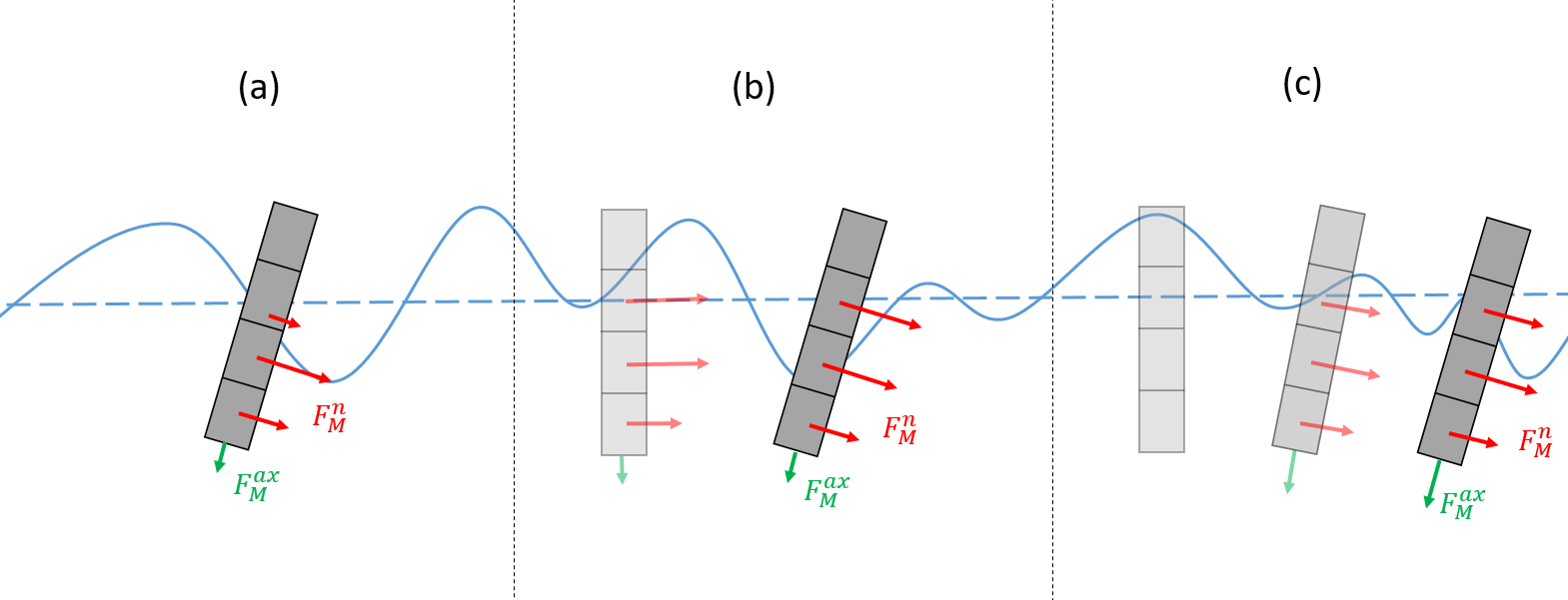
Fig. 14 Options in QBlade to consider the wave elevation and kinematics. (a) local instantaneous values; (b) values at the initial undisplaced position; (c) values at a low-passed position of the element.

The first option shown in Fig. 14 (a) is the wave kinematics and elevation at the local instantaneous position of the cylinder. In this example, the cylinder has been divided into four sub-elements. The lower two are fully submerged and one sub-element is partially submerged. The second option in Fig. 14 (b) is using the wave elevation and kinematics at the initial position of the sub-element. This option allows a coherent theoretical assumption of small oscillations around a steady positon when Morison forces are used in conjunction with a linear potential flow model (see Linear Potential Flow Theory). The third option uses the wave elevation and kinematics at a low-passed position of the sub-element (Fig. 14 (c)). This allows for an assumption of small oscillations around a steady state for an element that as drifted from its initial position due to an acting force such as and aerodynamic thrust or sea current hydrodynamic force.

1(1,2)

O. M. Faltinsen. Sea Loads on Ships and Offshore Structures. Cambridge University Press, 1993.

2

IEC61400-3-1 Standard. IEC 61400-3-1: Wind Energy Generation Systems - Part 3-1: Design Requirements for fixed offshore wind turbines. Standard, International Electrotechnical Commission, Geneva, Switzerland, 2019.

3(1,2)

USFOS Reality Engineering. USFOS Theory, Description of use and Verification Manual. https://www.usfos.no/manuals/usfos/theory/documents/Usfos_Hydrodynamics.pdf, 2021. [Online; accessed 2021-11-21].