Wave Generator Overview

Fig. 180 The wave generation module in QBlade’s main tool bar.
If an offshore simulation where the consideration of wave excitation is being carried out, it is necessary to provide the information about the sea sate in the form of a wave field. The field may either consist of a single wave train (regular wave) or multiple, superpositioned regular waves - (irregular waves). Both types may be generated directly in QBlade. A third possibility is the definition of a prescribed sea state, allowing the user to import externally generated wave fields. The three functionalities are described in more detail below. The underlying theory implemented in QBlade is described in the Waves section of the theory guide.
Any wave field generated in QBlade requires that a new wave is created by selecting this option in the Controls box. This opens the Linear Waves dialogue, where the wave generation options are displayed. In the Main Seastate Parameters box, the wave train is defined (amplitude and frequency). The Equal Energy Frequency Discretization box allows the user to tune the discretization parameters of the energy spectrum. Finally, the Equal Energy Directional Discretization box lets the user define directional properties of the wave.
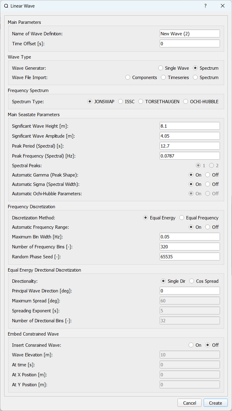
Fig. 181 The wave generator dialog in QBlade.
Regular Linear Wave
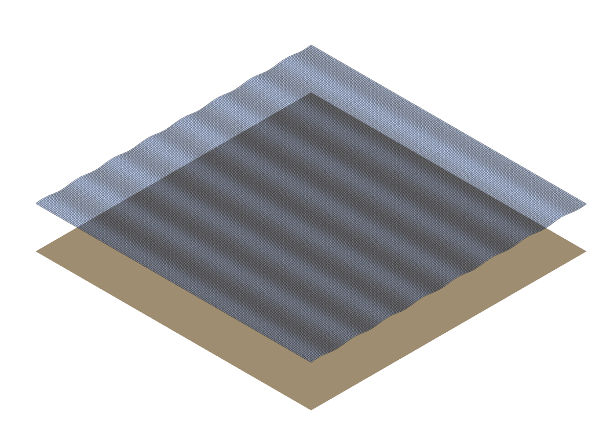
Fig. 182 Visualization of a regular wave.
To generate a regular wave, the wave type Regular Linear has to be chosen in the Linear Wave dialogue. The user now has the option to characterize the single wave train with the remaining available inputs. These parameters define the shape and direction of an Airy wave (see Linear Wave Theory).
Main Parameters
Time Offset: Time shift of the generated wave signal
Significant Wave Height: Height of wave train to be generated (directly linked to amplitude)
Significant Wave Amplitude: Amplitude of the wave (directly linked to wave height)
Peak Period: Period of the wave (directly linked to wave frequency)
Peak Frequency: Frequency of the wave (directly linked to the wave period)
Equal Energy Directional Discretization
Principal Wave Direction: Incoming wave direction
Regular Nonlinear Wave
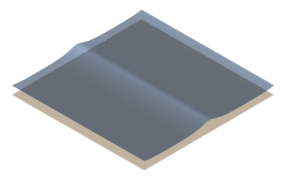
Fig. 183 Visualization of a regular nonlinear wave.
To generate a regular nonlinear wave, the wave type Regular Nonlinear has to be chosen in the Linear Wave dialogue. The user now has the option to characterize the nonlinear wave with the remaining available inputs. These parameters define the shape and direction of a nonlinear Streamfunction Wave. The Streamfunction waves are automatically generated using the CN-Stream library from LHEAA (see the work of G. Ducrozet et al. 1)
Main Parameters
Time Offset: Time shift of the generated wave signal
Significant Wave Height: Height of wave train to be generated (directly linked to amplitude)
Significant Wave Amplitude: Amplitude of the wave (directly linked to wave height)
Peak Period: Period of the wave (directly linked to wave frequency)
Peak Frequency: Frequency of the wave (directly linked to the wave period)
Equal Energy Directional Discretization
Principal Wave Direction: Incoming wave direction
Please note that nonlinear waves cannot be used to obtain hydrodynamic forces from Linear Potential Flow Theory , but are only suited to model Morison Equation based hydrodynamic forces.
Irregular Linear Wave
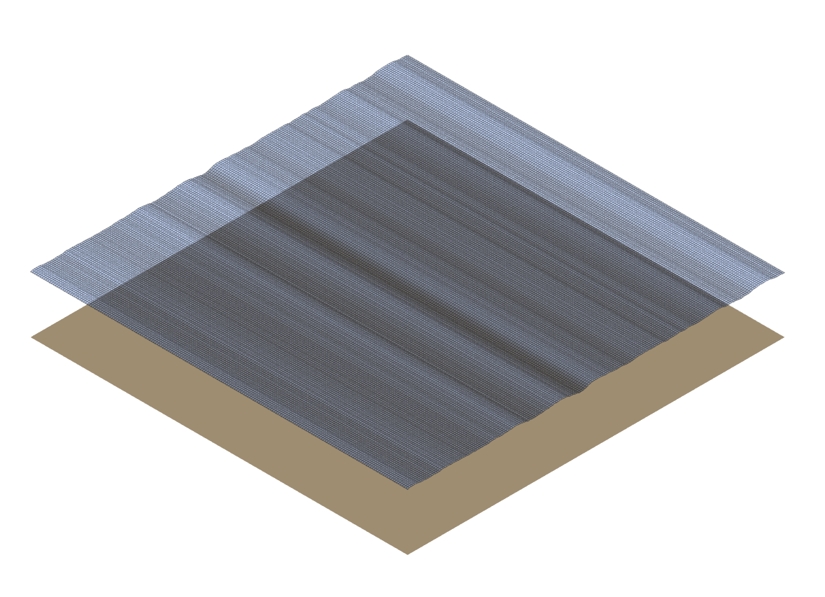
Fig. 184 Visualization of an irregular wave.
To generate an irregular wave, the wave type Irregular Linear has to be chosen. The user is now given the option to characterize the wave with the remaining available inputs. In addition to the wave train characterization discussed above, spectra discretization options can be specified.
Main Parameters
Time Offset: Time shift of the generated wave signal
Significant Wave Height: Wave height defining shape of the wave spectrum (directly linked to amplitude)
Significant Wave Amplitude: Wave amplitude defining shape of the wave spectrum (directly linked to height)
Peak Period: Peak period of the wave spectrum (directly linked to wave frequency)
Peak Frequency: Peak frequency of the wave spectrum (directly linked to the wave period)
Automatic Gamma: Automatic or manual definition of peak shape factor of the spectrum
Automatic Sigma: Automatic or manual definition of the spectral width parameter
Frequency Discretization
Discretization Method: The options are equal energy or equal frequency discretization of the wave spectrum
Maximum Bin Width: Maximum frequency range of the spectrum discretization.
Number of Frequency Bins: Resolution of frequency discretization of the energy spectrum.
Random Phase Seed: The random seed assigning the wave component phase data.
Equal Energy Directional Discretization
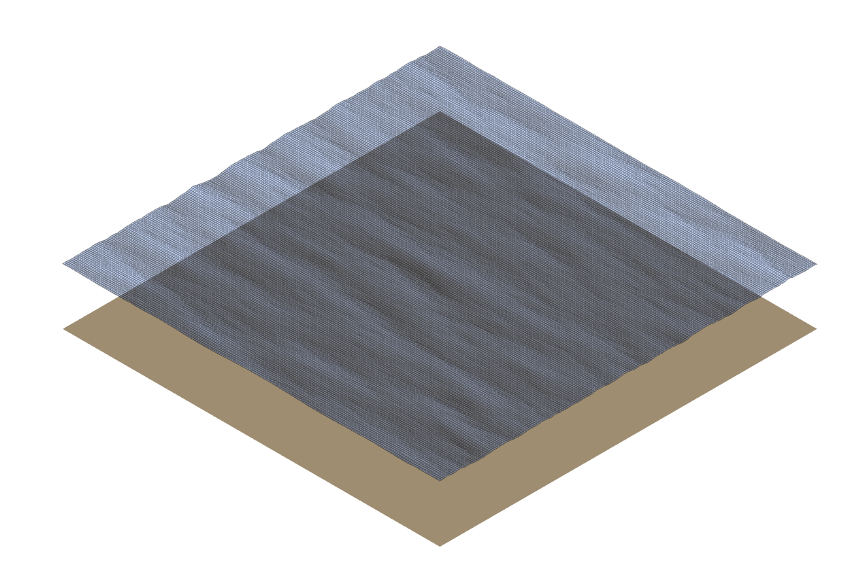
Fig. 185 Visualization of an irregular multi-directional wave.
Either a unidirectional irregular wave (Single Dir) or multidirectional wave (Cos Spread) can be created
Principal Wave Direction: Definition of the wave direction (unidirectional spectrum) or of the principal direction of the cosine spectrum.
Maximum Spread: Definition of the width of the cosine spectrum.
Spreading Exponent: Shape defining parameter for the directional spectrum
Number of Directional Bins: Resolution of angular discretization of the directional spectrum.
Embedded Constrained Wave
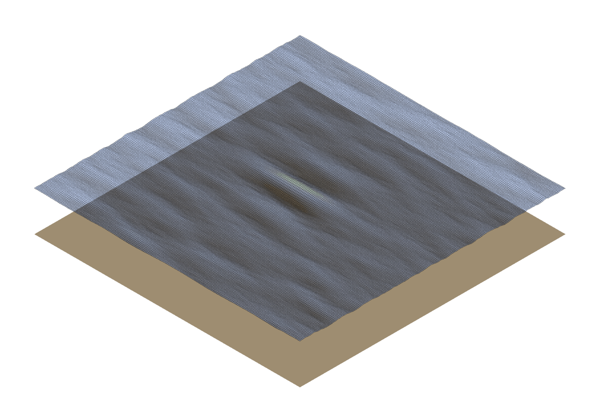
Fig. 186 A 30m constrained wave embedded in an irregular multi-directional wavefield.
QBlade also allows to embed a constrained wave into an irregular wavefield. This process is based on the NewWave method of Taylor 2 and follows the implementation that is as laid out in L. Wang, J. Jonkman, G. Hayman, A. Platt, B. Jonkman, A. Robertson3. The main use of this functionality is to reduce the required simulation time until a design wave event occurs. The extreme wave that is embedded hereby is conditioned on the underlying wave spectrum and is indistinguishable from a naturally occurring extreme wave.
It is highly suggested to use an Equal Frequency discretization, with sufficient wave trains when embedding a constrained wave.
Wave Elevation: The elevation of the embedded wave
At Time: The time at which the extreme wave occurs
At X Position: The X position at which the extreme wave occurs
At Y Position: The Y position at which the extreme wave occurs
Furthermore, it is possible to copy-paste a nonlinear regular wave over the constrained wave. This process is carried out in a similar way as described in the work by P. J. Rainey at al. 4. It is only possible to copy-paste a nonlinear wave over a constrained wave in an unidirectional wavefield. The user has to specify the following parameters of the embedded nonlinear wave:
Nonlinear Wave Height: The wave height of the pasted nonlinear wave
Nonlinear Wave Period: The period of the nonlinear wave
Please note that the Nonlinear Wave Height parameter is not the same as the Wave Elevation parameter that was specified for the constrained wave. The actual wave elevation of the pasted nonlinear wave also depends on other factors, such as the water depth.
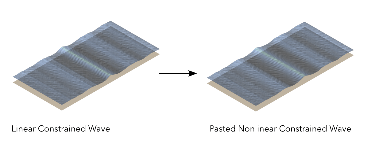
Fig. 187 An example of a nonlinear regular wave, pasted over a linear constrained wave in an irregular unidirectional wavefield.
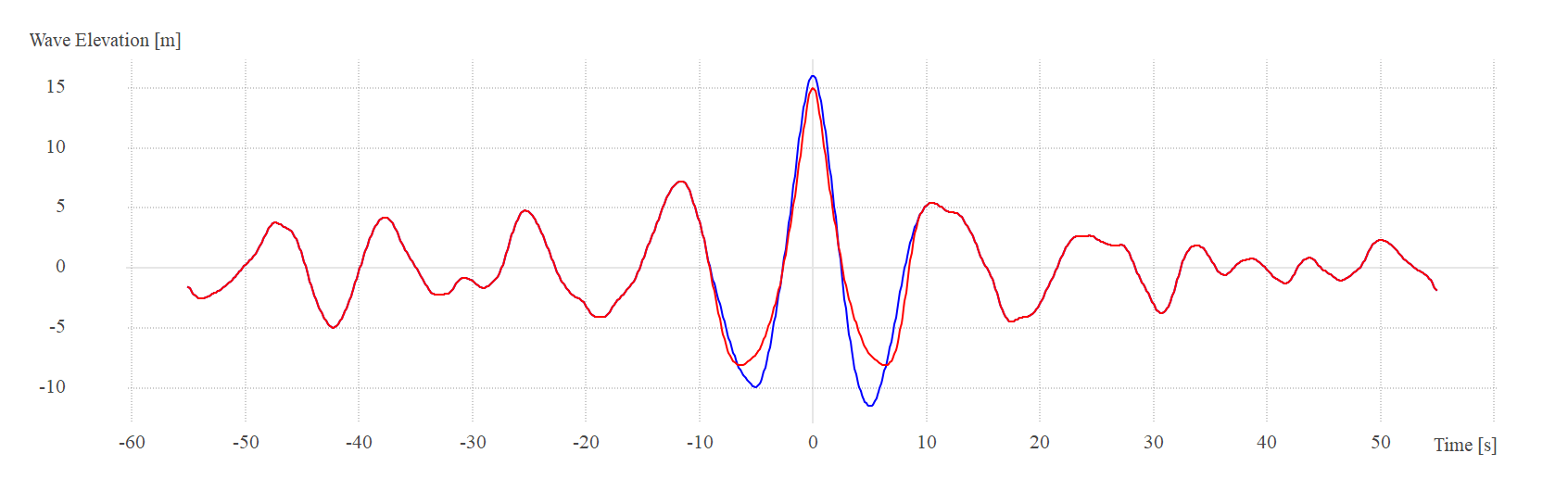
Fig. 188 Timetrace of wave elevation of the pasted nonlinear regular wave (in red), pasted over a linear constrained wave (in blue).
Nonlinear wave models in offshore wind turbine simulations offer enhanced accuracy by more realistically representing extreme sea states and complex wave interactions. The technique of pasting nonlinear waves into linear seas enables precise analysis of specific severe wave conditions without requiring extensive simulations to encounter such events naturally. This leads to more accurate predictions of structural loads, crucial for ensuring the safety and structural integrity of turbines, and facilitates more robust turbine design and risk assessment under challenging conditions.
Please note that nonlinear waves cannot be used to obtain hydrodynamic forces from Linear Potential Flow Theory , but are only suited to model Morison Equation based hydrodynamic forces.
Higher-Order Spectral Waves (HOS)
QBlade offers full integration with the Grid2Grid framework 56 to import and use nonlinear Higher-Order Spectral (HOS) wavefields in time-domain simulations. This coupling enables advanced modelling of wave kinematics and their interactions with floating and fixed offshore wind turbines. The underlying HOS methodology has been developed at École Centrale Nantes (LHEEA) 7, and the interpolation tool Grid2Grid is actively maintained within the LHEEA GitLab ecosystem..
Note
QBlade supports both HOS-Ocean and HOS-NWT datasets through this interface.
Loading HOS Wavefields
To use a HOS wavefield in QBlade, the user must provide:
A
.datfile containing the HOS wave simulation output.A corresponding
.jsonGrid2Grid configuration file.
The .json file describes the spatial interpolation grid for the HOS data. It is important to correctly set the mode parameter to either:
HOSOcean(for .dat files generated with HOS-Ocean),or
HOSNWT(for files from HOS-NWT).
Note
The
isAccelerationoption to in the.jsonfile is automatically set totruewithin QBlade.The
filePathvariable in the.jsonfile is automatically updated by QBlade based on the selected.datfile. Users do not need to modify this manually.Once loaded, the
.datfile is fully serialized into QBlade’s runtime database and stored for subsequent simulations.
Linearization of the HOS Field
QBlade allows two options when using HOS wavefields:
Fully nonlinear wave field — the original HOS data is directly sampled at runtime for:
Wave elevation
Velocity
Acceleration
Linearized wavefield — for each turbine instance in the simulation, a local linearization of the wavefield is automatically performed at simulation start. This local linearization is then used for:
Wave elevation
Velocity
Acceleration
When the Fully nonlinear wave field* option is used the elevation, velocity and acceleration data is sampled directly from the nonlinear HOS data, for Linear Potential Flow Theory based calculations, a local linearization of the HOS data is employed. The linearization occurs around the initial global position of each turbine. If the turbine is floating and may significantly shift position during simulation, it is recommended to apply an offset using the HOSOFFSET keyword in the turbine’s substructure file to align the linearization closer to the equilibrium position.
Example usage of the HOSOFFSET directive in a substructure input file:
HOSOFFSET
100 200 0
This adds an offset of +100 m in the global x-direction and +200 m in the global y-direction to the linearization origin.
FFT Conversion Parameters
An FFT-based routine is used to linearise the HOS wave-elevation signal. Five user-controlled settings govern how the time-domain record is decomposed into its linear frequency components:
Low cut-off frequency [Hz] and high cut-off frequency [Hz] delimit the frequency band that will be retained after filtering.
Signal sampling rate [Hz] specifies the temporal resolution of the input record and therefore the maximum resolvable frequency.
Amplitude threshold [m] suppresses spurious components whose amplitudes fall below the chosen value.
Window tapering [0 – 1] applies a Hann-type window to the time series; a value of 0 leaves the signal untouched, whereas 1 applies full tapering to minimise spectral leakage.
HOS Field Configuration Parameters
The following parameters must be specified when loading a HOS wavefield into QBlade:
Ref. Pos. X (in model scale) [m]
Ref. Pos. Y (in model scale) [m]
Defines the reference position in the unscaled (model) coordinate system. The HOS field will be centered around this point. Note that these coordinates are not scaled by the Froude number.
- Froude Scale [-]:
A user-defined Froude scaling factor used to scale the HOS wavefield to full scale. This allows loading wave tank (model scale) data and scaling it appropriately.
Use Nonlinear Field:
If selected, QBlade will sample the fully nonlinear HOS field for use with Morison elements. For potential flow elements, QBlade always uses the corresponding linearized local wavefield.
Principal Wave Direction [deg]:
By default, QBlade assumes that waves propagate in the global x-direction (0°). Users can override this by specifying a different principal direction.
Important
The linearization procedure assumes a uni-directional wavefield, with waves traveling in a consistent direction. The system assumes that direction to be 0° unless specified otherwise.
Import Components
By selecting this option the user can import a wave using wave component data.
when this option is selected a button appears Import Components File which allows the user to import a .txt file containing the wave component information.
This file must contains frequency [Hz], amplitude [m], phase [deg] and direction [deg] information of the wavefield in four columns.
This data represents the frequency domain information of the wave. This is inverse Fourier-transformed in order to specify a time-series of the wave data.
Once calculated, the button View Wave File appears allowing the user to visually check the imported data.
Import Timeseries
By selecting this option the user can import a wave using a time series of the wave height. A discrete Fourier transform (DFT) is applied to the timeseries in order to represent the data in the frequency domain. An inverse Fourier transform (IFT) is then applied to the Fourier coefficient in order to recreate the time-series data. A set of parameters must be specified for the DFT which gives the user some control of the wave components that are generated by the DFT. These parameters include:
Low Cut-Off Frequency: The minimum frequency considered in the DFT, below which wave components are discarded (approximately low-pass filtering).
High Cut-Off Frequency: The maximum frequency considered in the DFT, above which wave components are discarded (approximately high-pass filtering).
Signal Sampling Rate: The frequency with which data from the time series is sampled before the DFT is performed. This allows the user to reduce the number of wave components that will be generated by the DFT.
Amplitude Threshold: The minimum wave component amplitude allowed after the DFT is performed. This allows the user to filter out wave components with insignificant amplitude and thereby helps to reduce the number of generated wave components.
Import and Export Functionality
QBlade allows the user to import and export wave fields either in the four column format described in Import Components or in a .Iwa format.
The .Iwa format contains all of the parameters necessary to define the time and frequency domain descriptions of a wave.
This functionality can be found in the menu toolbar below the Wave tab.
Wave Definition ASCII File
An exemplary .lwa file is shown below:
----------------------------------------QBlade Wave Definition File-------------------------------------------------
Generated with : QBlade EE v2.0.8.7_beta windows
Archive Format: 310038
Time : 12:31:03
Date : 19.05.2025

----------------------------------------Object Name-----------------------------------------------------------------
New Wave                                           OBJECTNAME         - the name of the linear wave definition object

----------------------------------------Main Parameters-------------------------------------------------------------
0.000                                              TIMEOFFSET         - the time offset from t=0s [s]
3                                                  WAVETYPE           - wave type: 0=TIMESERIES, 1=COMPONENT, 2=SINGLE, 3=JONSWAP, 4=ISSC, 5=TORSETHAUGEN, 6=OCHI_HUBBLE, 7=CUSTOM_SPECTRUM, 8=STREAMFUNCTION, 9=HOS
8.100                                              SIGHEIGHT          - the significant wave height (Hs) [m]
12.700                                             PEAKPERIOD         - the peak period (Tp) [s]
true                                               AUTOGAMMA          - use gamma according to IEC (bool): 0 = OFF, 1 = ON (JONSWAP & TORSE only) [bool]
1.000                                              GAMMA              - custom gamma (JONSWAP & TORSE only)
true                                               AUTOSIGMA          - use sigmas according to IEC (JONSWAP & TORSE only) [bool]
0.070                                              SIGMA1             - sigma1 (JONSWAP & TORSE only)
0.090                                              SIGMA2             - sigma1 (JONSWAP & TORSE only)
0                                                  DOUBLEPEAK         - if true a double peak TORSETHAUGEN spectrum will be created, if false only a single peak (TORSE only)
true                                               AUTOORCHI          - automatic OCHI-HUBBLE parameters from significant wave height (OCHI only) [bool]
0.077                                              MODFREQ1           - modal frequency 1, must be "< modalfreq1 * 0.5" (OCHI only)
0.133                                              MODFREQ2           - modal frequency 2, should be larger than 0.096 (OCHI only)
6.804                                              SIGHEIGHT1         - significant height 1, should be larger than height 2 (OCHI only)
4.374                                              SIGHEIGHT2         - significant height 2 (OCHI only)
3.000                                              LAMBDA1            - peak shape 1 (OCHI only)
0.932                                              LAMBDA2            - peak shape 2 (OCHI only)

----------------------------------------Frequency Discretization ---------------------------------------------------
0                                                  DISCTYPE           - frequency discretization type: 0 = equal energy; 1 = equal frequency
true                                               AUTOFREQ           - use automatic frequency range (f_in = 0.5*f_p, f_out = 10*f_p) [bool]
0.039                                              FCUTIN             - cut-in frequency
0.787                                              FCUTOUT            - cut-out frequency
0.050                                              MAXFBIN            - maximum freq. bin width [Hz]
320                                                NUMFREQ            - the number of frequency bins
65535                                              RANDSEED           - the seed for the random phase generator range [0-65535]

----------------------------------------Directional Discretization (Equal Energy)-----------------------------------
0                                                  DIRTYPE            - the directional type, 0 = UNIDIRECTIONAL, 1 = COSINESPREAD
0.000                                              DIRMEAN            - mean wave direction [deg]
60.000                                             DIRMAX             - directional spread [deg]
5.000                                              SPREADEXP          - the spreading exponent
32                                                 NUMDIR             - the number of directional bins

----------------------------------------Embedded Constrained Wave --------------------------------------------------
false                                              EMBEDWAVE          - add a constrained wave [bool]
10.00                                              EMBEDELEV          - the wave elevation of the embedded wave [m]
0.00                                               EMBEDTIME          - the time at which the embedded wave occurs [s]
0.00                                               EMBEDXPOS          - the x-position at which the embedded wave occurs [m]
0.00                                               EMBEDYPOS          - the y-position at which the embedded wave occurs [m]
false                                              PASTESTREAM        - paste a streamfunction wave over the embedded linear wave [bool]
8.10                                               SIGHEIGHTSTREAM    - the significant height of the streamfunction wave [m]
12.70                                              PERIODSTREAM       - the period of the streamfunction wave [s]

----------------------------------------FFT Parameters (for sampling time series or HOS data)-----------------------
0.020                                              FFTCUTIN           - only frequencies above this value are used from the FFT
0.700                                              FFTCUTOUT          - only frequencies below this value are used from the FFT
20.000                                             FFTSAMPLE          - the timeseries is sampled with this rate before the FFT is carried out
0.001                                              FFTTHRESH          - amplitudes below the threshold will not be used to create wave components
0.100                                              TUKEYALPHA         - Tukey window shape: 0 = rectangular, 1 = Hann, values define taper amount in [0â??1]

----------------------------------------HOS Interface --------------------------------------------------------------
                                                                                                   HOSJSON            - the grid2grid JSON file [-]
                                                                                                   HOSDATA            - the grid2grid HOS data file [-]
0.0000                                             HOSX               - HOS wavefield neutral position x [m]
0.0000                                             HOSY               - HOS wavefield neutral position y [m]
1.0000                                             HOSFROUDE          - HOS wavefield Froude scale [-]
true                                               HOSNONLINEAR       - during simulations use the nonlinear HOS field for Morison elements and elevation
Merged Waves
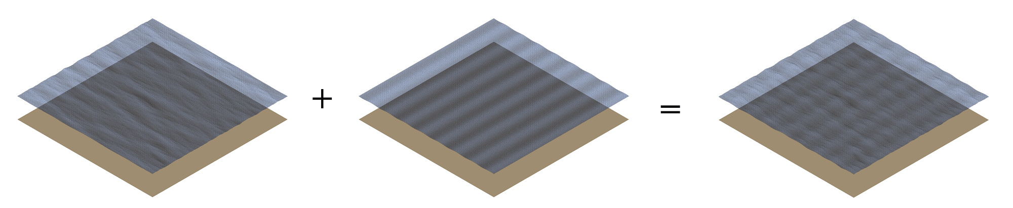
Fig. 189 Visualization of a new wave merged from an irregular and a regular wave.
It is also possible to merge two or more linear wave definitions to create a new merged wave. The merged wave is a simple superposition of the wave components of all merged waves. The main purpose for this option is to allow the user to generate seastates that are caused both by swell and wind coming from different directions. If both spectra (swell / wind) and their direction are known a merged wave can simply be created by merging both wave definitions.
The merge wave dialog is available from the top menu, shown in Fig. 190.
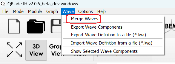
Fig. 190 The merged wave option in the top wave menu.
Merged Wave Definition ASCII File
A merged wave definition can also be exported to or imported from a simple ASCII format, that is shown below.
----------------------------------------QBlade Wave Definition File-------------------------------------------------
Generated with : QBlade CE v2.0.6_beta_dev windows
Archive Format: 310012
Time : 12:34:36
Date : 18.05.2023

----------------------------------------Object Name-----------------------------------------------------------------
New_Merged_Wave                          OBJECTNAME         - the name of the linear wave definition object

----------------------------------------Main Parameters-------------------------------------------------------------
2                                        MERGEDWAVES        - the number of linear waves that are merged in this wave
regular_wave.lwa                         WAVE_1             - the filenames of the waves that are merged
irregular_wave.lwa                       WAVE_2             - the filenames of the waves that are merged
- 1
Guillaume Ducrozet, Benjamin Bouscasse, Maïté Gouin, Pierre Ferrant, and Félicien Bonnefoy. Cn-stream: open-source library for nonlinear regular waves using stream function theory. 2019. arXiv:1901.10577.
- 2
P. H. Taylor. with the extremesof a Gaussian process. J. Vib. Acoustics, 1997.
- 3
L. Wang, J. Jonkman, G. Hayman, A. Platt, B. Jonkman, A. Robertson. Recent Hydrodynamic Modeling Enhancements in OpenFAST. NREL, 2022.
- 4
P J Rainey and T R Camp. Constrained non-linear waves for offshore wind turbine design. Journal of Physics: Conference Series, 75(1):012067, jul 2007. URL: https://dx.doi.org/10.1088/1742-6596/75/1/012067, doi:10.1088/1742-6596/75/1/012067.
- 5
École Centrale Nantes – LHEEA. Grid2grid – interpolation tool for hos wave fields. https://gitlab.com/lheea/Grid2Grid, 2025. Accessed 19 May 2025.
- 6
Y. M. Choi, M. Gouin, G. Ducrozet, B. Bouscasse, and P. Ferrant. Grid2grid: hos wrapper program for cfd solvers. arXiv, 1801.00026:1–17, 2017. URL: https://arxiv.org/abs/1801.00026, doi:10.48550/arXiv.1801.00026.
- 7
G. Ducrozet, F. Bonnefoy, D. Le Touzé, and P. Ferrant. Hos-ocean: open-source solver for nonlinear waves in open ocean based on high-order spectral method. Computer Physics Communications, 203:245–254, 2016. doi:10.1016/j.cpc.2016.02.017.