Linear Wave Theory

Linear wave theory (also referred to as Airy waves in the literature) may be applied when the sea water is assumed to be incompressible, inviscid and the fluid motion is irrotational. In addition to this is it assumed that the wave steepness is very small. Subsequently, a velocity potential can be used to describe the velocity vector (u,v,w) of a water particle at an arbitrary position (x,y,z) at any time (t) Energy1. Following these assumptions, the linear wave model in QBlade is implemented through the following set of equations. The velocity potential for finite depth may be expressed as

\[\begin{align} \Theta(x,y,z,t) = -\frac{gA}{\omega} \frac{cosh(k(z+h))}{cosh(kh)}cos(\omega t - kx) \end{align}\]

where,

• \(\Theta\) is the velocity potential,

• \(g\) is the graviational acceleration,

• \(A\) is the wave amplitude,

• \(\omega\) is the ciruclar frequency,

• \(h\) is the water depth,

• \(t\) is the time,

• \(x,y,z\) are Cartesian coordinates,

• \(k\) is the wave number.

The wave number k may be be expressed through the approximation of the dispersion relationship Guo2

\[\begin{align} k = \frac{\omega^2}{g}\Bigg(1-e^{-\omega \sqrt{\frac{h}{g}}^\frac{5}{2}}\Bigg)^{-\frac{2}{5}}. \end{align}\]

For infinite water depth the velocity potential is defined as:

\[\begin{align} \Theta(x,y,z,t) = -\frac{gA}{\omega} e^{kz} cos(\omega t - kx). \end{align}\]

Regular Waves

The wave elevation of a regular wave train at any position of the free surface at a given time t is defined by

\[\begin{align} \zeta (x,y,t) = A sin(kX-\omega t) \end{align}\]

where,

• \(\zeta\) is the wave elevation,

• \(X\) is the ordinate in wave direction defined as \(X = xcos(\Theta) +ysin(\Theta)\).

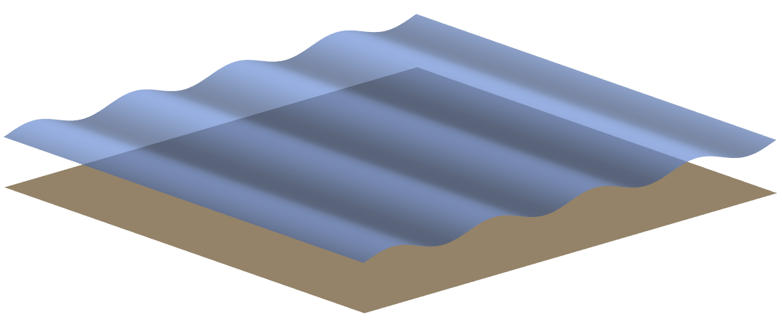
Fig. 22 Regular wave field created in QBlade

Unidirectional Irregular Waves

Irregular wave fields in QBlade belong to a short-term description of the sea, meaning that the significant wave height and the mean wave period are assumed to be constant over the considered time Faltinsen3. The irregular wave field is created through a linear superposition of N different linear waves trains. Each one of these wave trains is described by an amplitude \(A_j\), a circular frequency \(\omega_j\) and a phase \(\epsilon_j\) (\(0 - 2\pi\)). Hence, the wave elevation of an irregular wave field propagating along one direction (x-axis in this case) can be expressed through the following equation.

\[\begin{align} \zeta(x,y,t) = \sum_{j}^{N_j} A_j sin(k_jx -\omega_j t + \epsilon_j) \end{align}\]

in which \(N_j\) is the number of wave trains.

The amplitude \(A_j\) is to be determined by discretizing a wave spectrum \(S(\omega)\) into bins corresponding to a frequency range \(\Delta \omega\) Faltinsen3.

\[\begin{align} \frac{1}{2}A_j^2 = S(\omega_j)\Delta \omega \end{align}\]

Two of the most commonly used wave spectra are the Pierson-Moskowitz (PM), also known as ISSC-spectrum, and the JONSWAP (JS) spectrum. The former was originally proposed for fully developed sea and the latter extends the PM-spectrum to include developing sea states Nestegård et al.4. The spectra are described by the following equations.

\[\begin{align} S_{PM} = \frac{5}{16}\bigg(\frac{f}{f_p}\bigg)^{-5}H_s^2 T_p e^{-\frac{5}{4}\bigg(\frac{f}{f_p}\bigg)^{-4}} \end{align}\]

and

\[\begin{align} S_{JS} = A_\gamma S_{PM}(\omega) \gamma^{e^{-\frac{1}{2}\bigg(\frac{f-f_p}{\sigma f_p}\bigg)^{2}}} \end{align}\]

where,

• \(T_p\) is the peak period,

• \(f_p\) is the peak frequency,

• \(H_s\) is the significant wave height,

• \(A_\gamma\) is a normalizing factor,

• \(\gamma\) is the peak shape parameter

• \(\sigma\) is the spectra width parameter

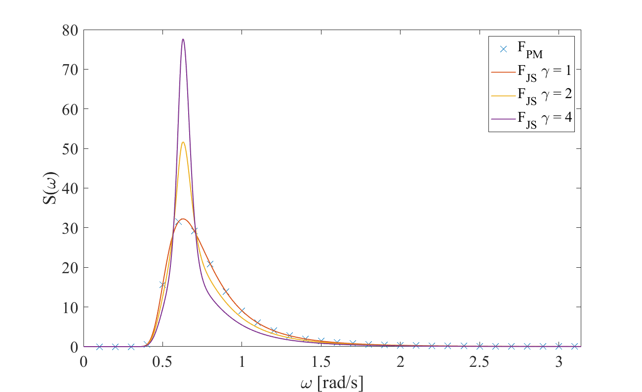
Fig. 23 Person-Moskowitz an JONSWAP spectra with different peak shape parameters \(\gamma\)

As visible in Fig. 23, the JONSWAP spectrum is a modification of the PM-spectrum by \(A_\gamma\) a normalizing factor, \(\gamma\) the peak shape parameter and \(\sigma\) the spectra width parameter Branlard5.

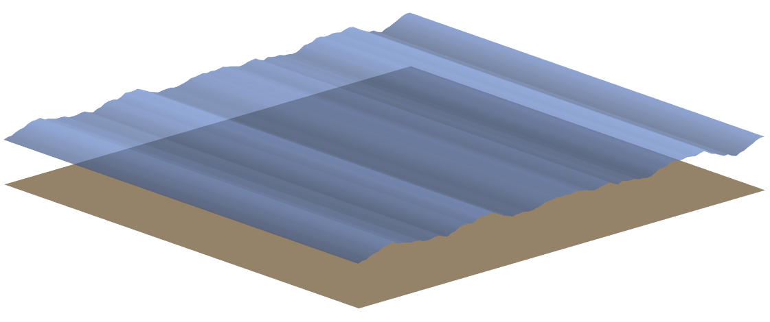
Fig. 24 Irregular wave field created in QBlade

Multidirectional Irregular Waves

A uni-directional wave spectrum \(S(\omega)\) may be augmented through a directional function \(D(\Theta)\) in order to create a multi-directional wave field Faltinsen3

\[\begin{align} S(\omega \Theta) = S(\omega) D(\Theta) \end{align}\]

where \(\Theta\) is the wave angle. The directional spectrum \(D(\Theta)\) is implemented in QBlade as defined in OrcaFlex6

\[\begin{align} D(\Theta) = C(s)cos^s(\Theta-\Theta_p) \end{align}\]

\(C(s)\) is a normalizing constant that is defined as

\[\begin{align} C(s) = \frac{\Gamma(\frac{s}{2}+1)}{\sqrt{(\pi)}\Gamma(\frac{s}{2}+\frac{1}{2})}. \end{align}\]

In this equation,

• \(s\) is the spreading exponent,

• \(\Theta_p\) is the principal wave direction,

When the directional spectrum is added, the equation of the wave elevation needs to be advanced by another summation term over the number of directions of the wave trains. Subsequently, the wave amplitude needs to be extended by the wave direction

\[\begin{align} \zeta(x,y,t) = \sum_{i}^{N_i}\sum_{j}^{N_j} A_{ij} sin(k_iX_j -\omega_i t + \epsilon_{ij}), \end{align}\]

\[\begin{align} \frac{1}{2}A_{ij}^2 = S(\omega_j,\Theta_j)\Delta \omega \Delta \Theta. \end{align}\]

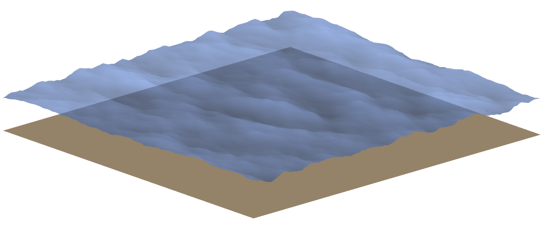
Fig. 25 Irregular, multi-directional wave field created in QBlade

1

DNV GL - Energy. Theory Manual Bladed. 2014. [Version 4.6].

2

Junke Guo. Simple and explicit solution of wave dispersion equation. Coastal Engineering, 45:71–74, 2002.

3(1,2,3)

O. M. Faltinsen. Sea Loads on Ships and Offshore Structures. Cambridge University Press, 1993.

4

Arne Nestegård, Marit Ronæss, Øistein Hagen, Knut Ronold, and Elzbieta Maria Bitner-Gregersen. On environmental conditions and environmental loads. In DNV Recommended Practice DNV-RP-C205. 05 2006.

5

E. Branlard. Generation of time series from a spectrum. Technical Report, Risø DTU National Laboratory for Sustainable Energy, 2010.

6

OrcaFlex. Directional spread spectrum. https://www.orcina.com/webhelp/OrcaFlex/Content/html/Wavetheory.htm#WaveSpreadingTheory, 2021.