Aerodynamic Modeling
This section covers all options that are related to the aerodynamic modelling of a turbine design. Covering wake models, dynamic stall models, geometry parameters and blade discretization.
Turbine Geometry
If no structural model is defined for this turbine object the turbine geometry is defined here. If a structural model is defined the geometry is defined within the structural model files.
Rotor Overhang: Sets the rotor overhang of the turbine object (see Fig. 95)
Tower Height: Definition of the tower height.
Tower Top/Bottom Radius: Defined the tower top and bottom radius. A linear interpolation is applied for all tower stations in between.
Rotor Shaft Tilt Angle: Sets the rotor shaft tilt angle (see Fig. 95).
Rotor Cone Angle: Sets the rotor cone angle (see Fig. 95).
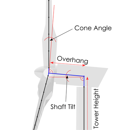
Fig. 95 Definition of turbine geometry parameters.
Aerodynamic Discretization
Blade Panels: Here the user can specify the number of blade panels and the type of spacing. A Linear spacing distributes the panels evenly over the blade length. A Cosine spacing results in a finer discretization near the blade ends (root and tip) and a slightly coarser discretization near the blade center. The option Table uses the aerodynamic blade definition table as a template for the aerodynamic discretization, thus the user can use this option for a fully customized blade discretization.
Aerodynamic Models
Dynamic Stall: The user can activate the use of a dynamic stall model. The options are: Off: No dynamic stall model is used. OYE: The OYE dynamic stall model is used, see OYE Model. ATEF: The ATEFlap unsteady aerodynamics model is used, see ATEFlap Model.
2 Point L/D Eval: This actives the two point lift and drag evaluation model, proposed by Li et al.1. The advantage of this two point evaluation is that lift and drag predictions for dihedral or coned wind turbine rotor are improved and the airfoil pitch rate is explicitly being taken into account by evaluating the angle of attack at the three-quarter chord point and then applying the aerodynamic coefficients at the quarter-chord point.
Himmelskamp Effect: The correction for the Himmelskamp effect can be activated here, see Himmelskamp Effect.
Tower Shadow: The Tower Shadow Effect can be activated or deactivated here, see Tower Influence.
Tower Drag Coeff.: Sets the drag coefficient that is used to model the Tower Shadow Effect. If a structural model is used for this turbine the tower drag coefficient is set in the 20th column of the structural tower data table, see Tower and Torquetube Euler Bernoulli and Timoshenko Datatable.
Wake Type
Here the user can choose between the Free Vortex Wake or the Unsteady BEM aerodynamic model. The Unsteady BEM model can only be used with HAWT turbine definitions.
Unsteady BEM
The Blade Element Momentum Method in QBlade is the default modeling option for HAWT (Horizontal Axis Wind Turbines). It has a low computational cost and good accuracy in most cases. The Unsteady BEM cannot be used to model VAWT (Vertical Axis Wind Turbines). To model a VAWT the Free Vortex Wake method must be used.
Unsteady BEM Options
Azimuthal Polar Grid Discretization: The polar grid is discretized into the chosen number of azimuthal sections. A value of 1 is equal to the BEM without a polar grid.
Include Tip Loss: This activates the classical BEM tip loss correction to account for a finite number of blades, see Glauert2.
Memory Effect Override Time: During the user-defined time interval, the time-lag constants used in the unsteady BEM formulation are temporarily increased by a factor of 20. This effectively enables a rapid convergence of the unsteady BEM solution toward a steady operating point. Once the override time has elapsed, the normal wake memory effect is reactivated.
The theory of the unsteady polar BEM is briefly described in Polar Grid.
Dynamic Wake Meandering (DWM)
The Dynamic Wake Meandering (DWM) model in QBlade provides a highly efficient, mid-fidelity approach to modeling wind turbine wakes. It captures the unsteady aerodynamics of wake meandering, deficit recovery, and wake-added turbulence without the extreme computational cost of a full CFD simulation.
This guide details the parameters available in the DWM configuration setup and provides recommendations for tuning your simulation, for more details on the theory see: Dynamic Wake Meandering Model
DWM Wake & Discretization Setup
These parameters control the spatial resolution and extent of the simulated wake. Higher resolution increases accuracy but demands more computational resources.
Total Wake Length (in D) [-] Sets the total downstream tracking distance of the wake, normalized by the rotor diameter (\(D\)). Wake planes that travel further downstream than this value are automatically deleted to save memory. Recommendation: 10 to 20 \(D\) is typical for farm simulations, depending on turbine spacing.
Number of Wake Planes [-] The maximum number of discrete 2D wake planes distributed over the total wake length. The spacing between planes is roughly
Total Wake Length / Number of Wake Planes. Recommendation: A value of 50-100 provides smooth downstream resolution.Max Wake Plane Width (in D) [-] Specifies the radial extent of the numerical grid for each wake plane. The plane must be wide enough to capture the fully expanded wake deficit. Recommendation: 3.0 \(D\) is usually sufficient. If simulating highly turbulent or heavily loaded conditions where wakes expand drastically, increase this value.
Wake Plane Radial Disc. [-] The number of radial grid points (\(N_{disc}\)) used to discretize the velocity profile from the center of the wake plane out to the Max Wake Plane Width. Recommendation: 40 is the default. Increasing this improves the resolution of the shear layer but slightly increases the cost of the viscous evolution step.
Wake Plane Update Dist. (in D) [-] The downstream propagation distance (\(\Delta\)) required before a wake plane’s velocity deficit profile is physically updated via the viscous Navier-Stokes solver. Recommendation: 0.1 \(D\) provides frequent, stable updates to the wake recovery profile.
Meandering & Spatial Averaging
To determine how the wake planes are pushed around by atmospheric turbulence, the local free-stream wind field is spatially averaged over a moving polar grid.
C Meander, Polar Grid Size (in D) [-] The diameter of the polar grid used to average the ambient wind field for evaluating the transverse (in-plane) meandering velocities. Recommendation: Typically set to 1.9 \(D\) to capture eddies larger than the rotor.
C Advect, Polar Grid Size (in D) [-] The diameter of the polar grid used to average the ambient wind field for evaluating the axial (out-of-plane) advection velocity. Recommendation: Typically set to 1.9 \(D\).
Polar Grid Measurement Points [-] The total number of measurement points distributed across the polar grid. Recommendation: 64 points provide a good balance between spatial coverage and wind field sampling speed.
Polar Grid Weighting [-] Specifies the spatial filter applied to the polar grid points during velocity averaging. Options:
UNIFORM(equal weight to all points),JINC1, orJINC2(Bessel-function filters that smoothly taper the influence of turbulence toward the grid edges).JINC2is highly recommended for standard DWM operation.Rotor Low Pass Filter Freq. [Hz] The cut-off frequency (\(f_c\)) of an exponential moving average low-pass time filter. This is used to smooth the rotor conditions (thrust, yaw) and advection velocities, preventing unphysical high-frequency jitter in the wake emission. Recommendation: 0.1 Hz is standard.
Wake Deficit & Recovery Models
These settings dictate how the velocity deficit is initialized immediately behind the rotor and how it mixes with the ambient air downstream.
Boundary Condition The model used to translate the blade axial induction (\(a\)) into the initial velocity deficit profile right behind the rotor. Options:
NONE(simple momentum),MADSEN,IEC, orKECK.MADSENandKECKare robust choices that account for initial stream-tube expansion.Viscosity Model The eddy-viscosity formulation used to solve the momentum equations during the wake evolution step. This dictates how fast the wake recovers. Options:
MADSEN,LARSEN,IEC, orKECK.Thrust Coefficient Ct [-] Used to calculate the initial deficit magnitude. Options: Choose Auto to compute this dynamically from the local blade aerodynamics at each time step, or Manual to override it with a constant value (e.g., 0.8).
Turbulence Intensity [-] The ambient turbulence intensity (\(TI\)) used by the viscosity models to determine atmospheric mixing. Options: Choose Auto to sample this dynamically from the inflow wind field, or Manual to override it.
Wake Deflection (Yaw & Tilt)
If the turbine is yawed or tilted relative to the inflow, the wake is deflected laterally or vertically.
Include Rotor Tilt If activated, the rotor’s tilt angle explicitly drives a vertical deflection of the wake planes.
Yaw Deflection Factor [1/deg] A tunable parameter for the lateral wake deflection correction, scaled by the yaw error. Recommendation: Default is -0.004.
Tilt Deflection Factor [1/deg] A tunable parameter for the vertical wake deflection correction, scaled by the tilt error. Recommendation: Default is -0.004.
DWM Added Turbulence Settings
Because the spatial averaging process intentionally filters out micro-scale turbulence, the high-frequency turbulence generated by the turbine’s shear layer must be artificially reintroduced to accurately model fatigue loads on downstream turbines.
Enable Added Turbulence Activates the micro-scale turbulence superposition model.
Added Turbulence Box The file path to a pre-generated synthetic wind field (e.g., a TurbSim .bts file). Important: This specific wind field must be generated with unit variance and isotropic turbulence, as it will be scaled dynamically by the DWM solver.
Added Turbulence km1 [-] The tuning parameter (\(k_{m1}\)) that scales the added turbulence based on the absolute magnitude of the local velocity deficit. Recommendation: 0.1234 (default baseline calibration).
Added Turbulence km2 [-] The tuning parameter (\(k_{m2}\)) that scales the added turbulence based on the radial velocity gradient (the shear layer intensity). Recommendation: 0.1234 (default baseline calibration).
Free Vortex Wake
The Lifting Line Free Vortex Wake method in QBlade yields an improved accuracy over the Unsteady BEM method, especially for unsteady operating conditions, such as changing inflow speed or direction or floating wind turbines, that are subjected to wave forces. This increased fidelity however comes at an increased computational cost. Furthermore, the number of settings that are required to setup this method is significantly larger than the BEM settings. All LLFVW modeling options are detailed in the following.
Wake Modelling
Wake Integration Type: This sets the velocity integration method for the wake nodes during the free wake convection step. EF: A simple 1st Order Euler Forward integration. PC: A 2nd Order Predictor Corrector integration method. PC2B: A second Order Predictor Corrector Backwards integration scheme.
Wake Rollup: This actives or deactivates the wake self-induction.
Include Trailing/Shed Vortices: This sets if trailing (streamwise) or shed (spanwise) vortices are generated at the blades trailing edge during every timepstep.
Wake Convection: The user can choose here which free-stream velocity contributes to the total convection velocity of the wake nodes. BL: The convection velocity is the mean boundary layer velocity (as a function of height). HH: The convection velocity is the constant hub-height velocity. LOC: The convection velocity is evaluated locally at each wake node position.
Wake Relaxation Factor: This factor can be used to relax the wake by blending out the starting vortex. The factor controls how long the wake is allowed to be after a given number of rotor revolutions or timesteps (depending on the Count Wake Length In setting). Such as a value of 0.5 allows for a wake length of 5 revolutions after the rotor has undergone 10 revolutions. A factor of 1 deactivates the blending.
First Wake Row Length Factor: This factor can be used to assign a shortened length to the newly created wake elements at the trailing edge so that the newly created shed vorticity is in closer proximity to the blade. A factor of 1 deactivates the shortening.
Max Num. Elements / Norm. Distance: These two values are used to cut-off the wake after a fixed number of vortex elements has been created (Max. Num. Wake Elements) or after a vortex element has reached a distance (normalized by rotor diameter) from the hub that is larger than Norm. Distance.
Wake Reduction Factor: This factor filters out wake elements that have a circulation smaller than the maximum circulation in the wake multiplied by this factor. In most cases this effectively removes shed vorticity that does not significantly affect the wake induction (see Fig. 96).

Fig. 96 Visualization of the wake reduction approach.
Count Wake Length In: This setting controls how the age of a vortex element is counted. Either as a number of rotor revolutions, or as a number of timesteps that have passed since the element was created.
Particle Conversion after [Revolutions/Timesteps]: (Only QBlade-EE) This setting controls when a vortex filament is converted into a vortex particle. If the vortex element has reached an age (in timesteps or revolutions) equal to this value it is converted into a particle.
Wake Zones N/1/2/3 in [Revolutions/Timesteps]: This setting controls the length of the different wake zones. The length is either counted in rotor revolutions or in timesteps, depending on the setting (Count Wake Length In). Each wake zone has a successively coarser discretization (depending on the Wake Zones Factor settings) to reduce the total number of free wake elements and thereby to speed up the simulation.
Streamwise Factor 1/2/3: These (integer) factors control by how much the wake is coarsened in the streamwise direction in between the different wake zones. A factor of 2 means that when transitioning from one zone to the next 2 trailing wake elements are merged into a single wake element to coarsen the wake resolution (see Fig. 97).
Spanwise Factor 1/2/3: These (integer) factors control by how much the wake is coarsenend in the spanwise direction between the different wake zones. A factor of 2 means that when transitioning from one zone to the next 2 shed wake elements are merged into a single wake element to coarsen the wake resolution in the spanwise direction (see Fig. 98).

Fig. 97 Visualization of the wake zoning approach and coarsening in the streamwise direction. For illustrative purposes the rotor does not rotate and the length of each wake zone is 50 timesteps.

Fig. 98 Visualization of the wake zoning approach and coarsening in the spanwise direction. For illustrative purposes the rotor does not rotate and the length of each wake zone is 50 timesteps.

Fig. 99 Visualization of the wake zoning approach and coarsening in the combined streamwise and spanwise direction. For illustrative purposes the rotor does not rotate and the length of each wake zone is 50 timesteps.
Vortex Modelling
Fixed Bound Core Radius (% Chord): This sets the fixed core radius of the bound blade vortices. Defined as a fraction of the local blade chord.
Initial Wake Core Radius (% Chord): This sets the initial core radius of the free vortices that are created at the blades trailing edge. Defined as a fraction of the local blade chord.
Turbulent Vortex Viscosity: This value is used in the vortex core growth model, see Vortex Core Desingularization.
Include Vortex Stretching: This option activates vortex stretching, see Vortex Core Desingularization.
Maximum Vortex Stretching Factor: After the cumulative vortex strain rate has reached a value larger than this factor it is automatically removed from the wake.
Turbine Gamma Iteration Parameters
Relaxation Factor: This relaxation factor is used when the blade circulation is updated during the circulation iteration.
Max. Epsilon for Convergence: The convergence criteria for the blade circulation.
Max. Number of Iterations: The maximum number of blade circulation iterations that will be carried out.
- 1
A. Li, M. Gaunaa, G. R. Pirrung, A. Meyer Forsting, and S. G. Horcas. How should the lift and drag forces be calculated from 2-d airfoil data for dihedral or coned wind turbine blades? Wind Energy Science Discussions, 2022:1–40, 2022. URL: https://wes.copernicus.org/preprints/wes-2021-163/, doi:10.5194/wes-2021-163.
- 2
H. Glauert. Airplane Propellers, chapter Aerodynamic Theory, pages 169–360. Springer Berlin Heidelberg, 1935. doi:10.1007/978-3-642-91487-4_3.