ATEFlap Model

To account for dynamic stall and unsteady aerodynamics the ATEFlap 1 model for 2D airfoil behavior has been integrated to be used with Lifting Line Free Vortex Wake simulations.

Note that the ATEFlap model has been specifically modified to be used with Lifting Line Free Vortex Wake simulations 2, it is currently not advised to use the ATEFlap model in simulations that use the Blade Element Momentum Method aerodynamic model.

The ATEFlap unsteady aerodynamics model consists of mainly two parts; an attached or potential flow model, as proposed by Bergami and Gaunaa 1, and the classical Beddoes-Leishman dynamic stall model with a custom formulation for vortex lift, as presented by Hansen and Gaunaa 3. The implemented ATEFlap model also accounts for unsteady lift contribution of active trailing edge flap deflections. In its implementation in QBlade the ATEFlap dynamic stall model is only applied within the angle of attack range of -50° to 50°.

Decomposed Polar Data

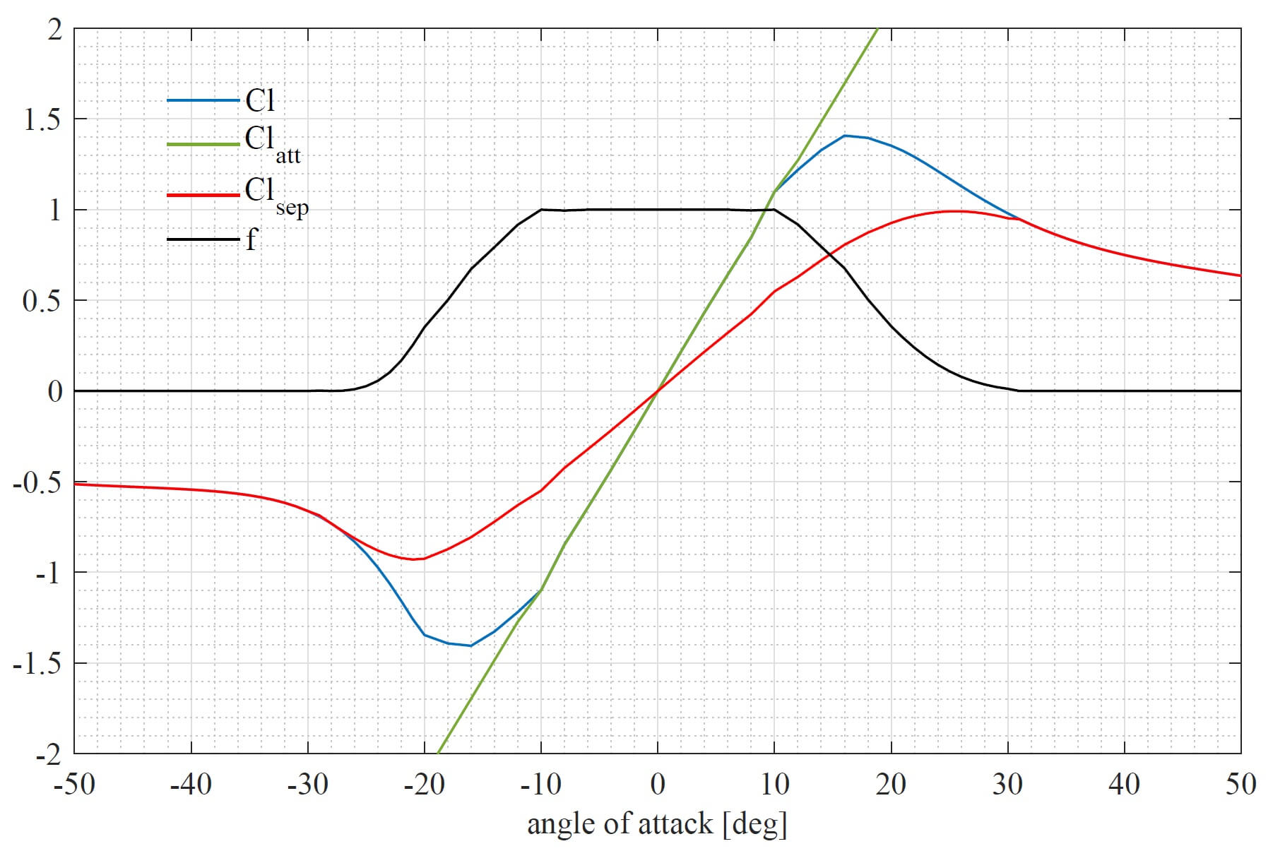
Fig. 9 Decomposition of static polar data.

The unsteady aerodynamics model is based on a decomposition of the static, two dimensional lift \(Cl_{st}\) into a fully attached \(Cl_{att}\) and a fully separated \(Cl_{sep}\) contribution. This is shown in Fig. 9. The contributions of the attached and the separated lift to the static lift are described by the following equation:

\[\begin{align} Cl_{st} = f Cl_{att} + (1-f) Cl_{sep}, \end{align}\]

where \(f\) represents the separation function.

A module to perform the decomposition of polar data has been integrated with QBlade’s airfoil data pre-processor (see Polar Decomposition).

Lift: Attached Flow Contribution

The potential flow model accounts for non-circulatory (added mass) effects, and circulatory lift which includes wake memory effects that play a role in the linear attached flow region. The added mass term models the forces due to the reaction of the fluid to the airfoil motion and the motion of its trailing edge flap:

\[\begin{align} Cl^{nc} = \pi\frac{b_{hc}}{V_\infty}\dot{\alpha}^{str} + \frac{F_{dydxLE}}{\pi}\frac{b_{hc}}{V_\infty}\dot{\beta}. \end{align}\]

\(b_{hc}\) denotes the half chord length of the airfoil, \(V_{\infty}\) the free stream velocity and \(\dot{\alpha}_{str}\) the pitch rate due to torsional deformation, \(F_{dxdyLE}\) is the deflection shape integral, a geometrical property depending on the airfoils shape (See Gaunaa’s work in 4) and \(\dot\beta\) the flap deflection rate.

The quasi steady lift component is the steady lift that is generated by the airfoil at the current angle of attack \(\alpha_{qs}\) and the current flap deflection \(\beta_{qs}\) obtained from the relative airfoil motion and free-stream velocity, but without the influence of shed wake vorticity:

\[\begin{align} Cl^{qs} = Cl^{att}(\alpha_{qs}, \beta_{qs}). \end{align}\]

The circulatory component of the lift coefficient is obtained by evaluating the attached lift coefficient at the effective angle of attack \(\alpha_{eff}\) with the effective flap angle \(\beta_{eff}\) (see 1 for details).

\[\begin{align} Cl^{circ}=Cl^{att}(\alpha_{eff}, \beta_{eff}). \end{align}\]

\(\alpha_{eff}\) is the angle of attack that arises of the airfoil interaction with its wake. Wake memory effects are caused by the influence of the trailing and shed vorticity in the wake on the quasi-steady angle of attack. Originally the ATEFlap model was formulated for BEM codes, so the downwash of the wake (which also causes the wake memory effect) is modeled with an effective angle of attack that is computed via step responses that are described by exponential indicial response functions 1. In QBlade’s implementation, the effective angle of attack is directly obtained as the induction from the free vortex wake formulation is already considered in the evaluation of the on-blade velocities.

It should be noted that the quasi steady angle of attack, which does not include the effect of wake vorticity, is not known in the free vortex wake formulation of QBlade. As the quasi steady angle \(\alpha_{qs}\) is needed for a later evaluation of the induced drag contribution it is computed by calculating the isolated contribution of the wake vorticity on the angle of attack, denoted as \(\alpha_{shed}\), separately. \(\alpha_{shed}\) is obtained by considering the induction of the total shed vorticity in the vicinity of the blade, up to \(8\) chord lengths away from the trailing edge. As the dynamic stall model is formulated for an isolated two-dimensional airfoil, it is necessary to limit the vortices that are involved in the evaluation of \(\alpha_{shed}\) to those in the vicinity of the blade to exclude the significant influence of the total shed vorticity from all previous time steps on the global flow field (this is especially important for VAWT simulations where the shed vorticity has a major contribution to the total induction field around the rotor). \(\alpha_{shed}\) is then used to calculate the quasi steady angle of attack from the effective angle of attack.

\[\begin{align} \alpha_{qs} = \alpha_{eff}-\alpha_{shed}. \end{align}\]

This extra treatment is necessary because the common unsteady aerodynamics models are formulated for BEM codes and use indicial functions. In QBlade, these functions are replaced by the free vortex wake model.

Lift: Separated Flow Contribution

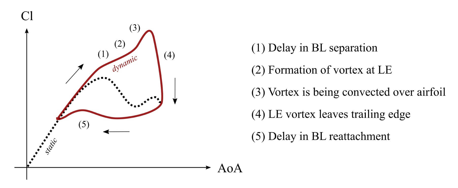
Fig. 10 The dynamic stall hysteresis loop.

The implementation of the Beddoes-Leishman dynamic stall model follows the procedure explained in 1. A schematic representation of the dynamic stall loop is shown in Fig. 10.

In QBlade, the dynamic stall effect is modeled by means of three contributions. The first contribution is the lagged potential lift (leading edge pressure time lag), obtained via a low pass filter function with the pressure time lag constant \(\tau_p\):

\[\begin{align} \dot{Cl}^{lag} = -\frac{V_{\infty}}{b_{hc}}\frac{1}{\tau_p}Cl^{lag}+\frac{V_{\infty}}{b_{hc}}\frac{1}{\tau_p}Cl^{pot}. \end{align}\]

In the equation above, \(Cl^{pot}\) represents the potential lift from the attached flow contribution:

\[\begin{align} Cl^{pot} = Cl^{circ} + Cl^{nc}. \end{align}\]

Using the lagged potential lift \(Cl^{lag}\) the second contribution can be calculated, namely the intermediate separation function. In this contribution, a separation function is calculated from the static separation function \(f\) (obtained via the polar decomposition) in combination with an equivalent angle of attack \(\alpha_{\ast}\) and flap angle \(\beta_{\ast}\) that are obtained with the help of \(Cl^{lag}\):

\[\begin{split}\begin{align} \alpha^{\ast} &= \frac{Cl^{lag}}{\frac{\partial Cl}{\partial \alpha}}+\alpha_0, \\ \beta^{\ast} &= \frac{Cl^{lag} - Cl^{lag}_{\beta=0}}{\frac{\partial Cl}{\partial \beta}}. \end{align}\end{split}\]

With the help of \(\alpha^{\ast}\) and \(\beta^{\ast}\), the third contribution can be calculated: the dynamic separation function. In this contribution, the dynamic separation function \(f^{dyn}\) is calculated by passing the intermediate separation function \(f(\alpha^{\ast},\beta^{\ast})\) through a low pass filter with the boundary layer lag constant \(\tau_f\):

\[\begin{align} \dot{f}^{dyn} = -\frac{V_{\infty}}{b_{hc}}\frac{1}{\tau_f}f^{dyn}+\frac{V_{\infty}}{b_{hc}}\frac{1}{\tau_f}f(\alpha^{\ast},\beta^{\ast}), \end{align}\]

The dynamic circulatory lift \(Cl^{circ,dyn}\) is then obtained by multiplying the dynamic separation function \(f^{dyn}\) with the fully attached \(Cl^{att}\) and the fully separated \(Cl^{sep}\) lift contributions that were obtained from the polar decomposition:

\[\begin{align} Cl^{circ,dyn} = Cl^{att}(\alpha_{eff},\beta_{eff})f^{dyn}+Cl^{sep}(\alpha_{eff},\beta_{eff})(1-f^{dyn}). \end{align}\]

Within the ATEFlap formulation for separated flow a term for modeling the vortex lift is included:

\[\begin{align} C_v = Cl^{circ,dyn}(1-\frac{(1+\sqrt{f^{dyn}})^2}{4}). \end{align}\]

However, it was found, especially when simulating VAWT with large fluctuations in angle of attack, that this term is prone to large fluctuations, often causing unrealistically large values for the total dynamic lift coefficient. Thus, in favor of robustness, it was decided to exclude this term from the calculation of total lift. The total lift, including the attached and separated flow contribution, but excluding the vortex lift, then equals:

\[\begin{align} Cl^{dyn} = Cl^{circ,dyn}+Cl^{nc}. \end{align}\]

Drag

The dynamic drag is evaluated from four contributions. These are: first, the steady drag at the effective angle of attack and the effective flap angle:

\[\begin{align} Cd^{eff} = Cd(\alpha_{eff},\beta_{eff}). \end{align}\]

Second, the drag induced from shed wake vorticity. It is obtained using the quasi steady angle of attack:

\[\begin{align} Cd_{ind}=Cl^{circ,dyn}(\alpha_{qs}-\alpha_{eff}). \end{align}\]

The third contribution is the induced drag contribution from the flap deflection. It is calculated according to:

\[\begin{align} Cd_{ind}^\beta=Cl^{circ,dyn}\cdot \frac{\frac{\partial Cl}{\partial\beta}}{\frac{\partial Cl}{\partial\alpha}}(\beta^{st}-\beta^{eff})f^{dyn}. \end{align}\]

The last contribution is the drag change caused through the separation delay:

\[\begin{align} Cd_{ind}^f = (Cd^{eff}-Cd(\alpha_0))\left[\frac{\left(1-\sqrt{f^{dyn}(\alpha^{\ast},\beta^{\ast})}\right)^2}{4}-\frac{\left(1+\sqrt{f^{st}(\alpha^{\ast},\beta^{\ast})}\right)^2}{4}\right]. \end{align}\]

The total drag is then computed as the sum of these contributions:

\[\begin{align} Cd = Cd^{eff}+Cd_{ind}+Cd_{ind}^\beta+Cd_{ind}^f. \end{align}\]

1(1,2,3,4,5)

Leonardo Bergami and Mac Gaunaa. ATEFlap Aerodynamic Model. Technical Report, DTU, 2012.

2

Juliane Wendler, David Marten, George Pechlivanoglou, Christian Oliver Paschereit, and Christian Navid Nayeri. An Unsteady Aerodynamics Model for Lifting Line Free Vortex Wake Simulations of HAWT and VAWT in QBlade. In Proceedings of ASME Turbo Expo 2016: Turbomachinery Technical Conference and Exposition. 2016.

3

Morten Hartvig Hansen, Mac Gaunaa, and Helge Aagaard Madsen. A Beddoes-Leishman type dynamic stall model in state-space and indicial formulation. Technical Report, DTU, 2004.

4

Mac Gaunaa. Unsteady two-dimensional potential flow model for thin variable geometry airfoils. Wind Energ., 13(December 2005):167–192, 2010. URL: https://doi.org/10.1002/we.377.