Polar Extrapolation Overview
The numerical models used by QBlade to calculate aerodynamic properties and forces require knowledge of the airfoil sectional properties. It is often the case that the polar data for an airfoil (which has previously been either defined or imported- see Airfoil Generation Overview) is only available for a certain range of angles of attack \(\alpha\), these we shall refer to as partial polars. It often occurs that as a result of the turbine architecture, geometry, operational state or other factors that \(\alpha\) values outside of this range are experienced by the airfoils of the turbine blade. For this reason, the blade creation module of QBlade requires that polars are defined for the full 360 \(^\text{o}\) \(\alpha\) range. It is therefore practical to have a methodology for extrapolating the partial polars. This is possible within QBlade using the polar extrapolation module. The module button in the main toolbar for this is shown in Fig. 54.

Fig. 54 The polar extrapolation module is represented by the 360 \(^\text{o}\) symbol in the QBlade main tool bar.
A range of options for generating or defining 360 \(^\text{o}\) polars are available in the polar extrapolation module. These are described in the following sections.
Viterna Extrapolation
The first option available to extrapolate airfoil polar data is the Viterna method. 1. The generated extrapolation is visualized in the graph section to allow for optimization. The following parameters can be tuned to improve the behavior of the polar:
Range of original polar: This determine which \(\alpha\) range of the polar is used for the interpolation.
CD90: Specifies the value of the drag coefficient at \(\alpha = 90^\text{o}\). This also influences the lift coefficient behavior.
St+, St-: These specify the positive and negative stall \(\alpha\) for the airfoil, respectively.
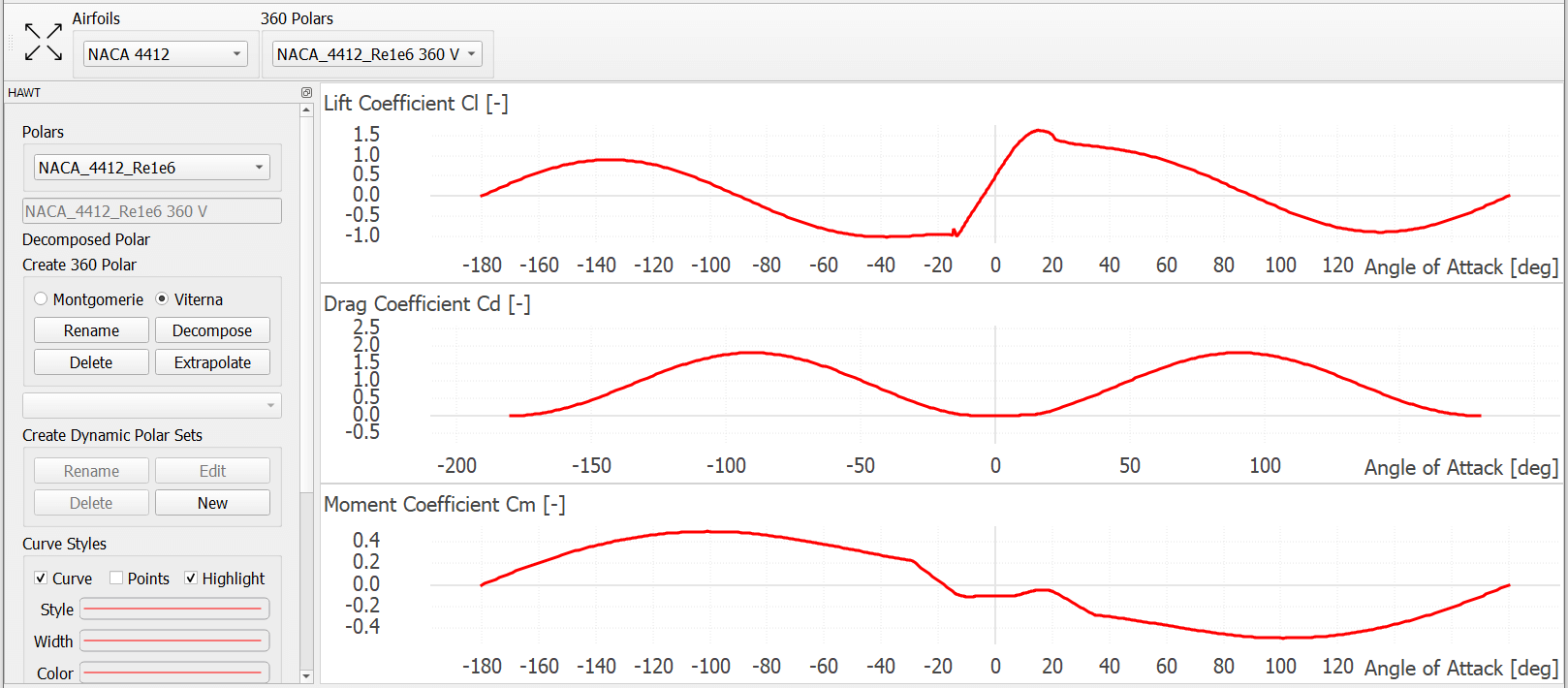
Upon generation the tuning parameters are specified such that they correspond to those recommended in Viterna 1. Once the polar is found to be suitable, this can be stored by clicking on the Save button. A full visualization of an airfoil extrapolation with the Viterna method is shown in Fig. 55.

Fig. 55 An airfoil extrapolation carried out using the Viterna method in QBlade.
Montgomery Extrapolation
The second option available to extrapolate airfoil polar data is the Montgomery method 2. This method is based on the assumption that the airfoil acts aerodynamically as a flat plat for high values of \(\alpha\). The generated extrapolation is visualized in the graph section to allow for optimization. The following parameters can be tuned to improve the behavior of the polar:
A+/B+: These are curve parameters corresponding to the positive \(\alpha\) range.
A-/B-: These are curve parameters corresponding to the negative \(\alpha\) range.
Slope: This is a matching parameter which ensures continuity of the curve slope.
CD90: Specifies the value of the drag coefficient at \(\alpha = 90^\text{o}\). This also influences the lift coefficient behavior.
Upon generation the tuning parameters are specified such that they correspond to those recommended in Montgomerie 2. Once the polar is found to be suitable, this can be stored by clicking on the Save button.
Polar Decomposition
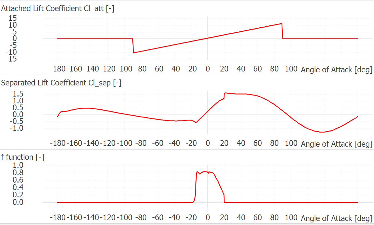
In the case that the ATEFlap Model dynamic stall model is to be applied for a simulation, then a decomposition of the airfoil must be carried out. This separates the the airfoil coefficients into fully attached and fully separated regimes, which are applied together with kinematic data to calculate the unsteady lift, drag or moment coefficients. In QBlade this decomposition is automatically performed during the polar extrapolation - or can be applied as a post processing to already extrapolated polars. Once the extrapolation has been carried out, the parameters of the decomposition can be visualized. The parameters are include:
Attached Lift Coefficient: The value of the lift coefficient for attached flows.
Detached Lift Coefficient: The value of the lift coefficient for detached flows and dynamic airfoils near the detachment point.
f function: The function which determines the fraction of the aforementioned lift contributions over the range of angles of attack.
A plot of these parameters, as generated for a NACA 4412 profile are shown in Fig. 56.

Fig. 56 Dynamics airfoil parameters for a NACA 4412 polar decomposition carried out in QBlade.
Dynamic Polar Sets
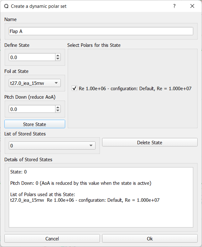
In QBlade dynamic polar sets can be used to model the changing states of flow control devices, such as trailing edge flaps. Dynamic polar sets allow to store polars that represents a series of states. For example: for a flap each state would correspond to a certain flap deflection angle. For each state multiple polars, covering a range of Reynolds numbers, may be stored. A dynamic polar set can then be assigned to an active element in the Blade and Rotor Design. The different states can then later be activated by the Turbine Controller Libraries or the Actuator Control Panel.
Fig. 57 shows the dialog to create dynamic polar sets.

Fig. 57 The dynamic polar set creator dialog.
Import and Export of 360 Polars
Much as is the case with non extrapolated polars, a range of import and export options exist so that external sources and files may be used to define 360 \(^\text{o}\) polars within QBlade. This is achieved by selecting the 360 Polar menu option.
Plain text format: These include either AeroDyn V13 files or XFoil formats (see Airfoil Generation Overview)
Multi Re polar file: The
.plrformat is the main format to import or export polar data. It can also be used to import polar data that is defined over a range of Reynolds numbers.
When a .plr file is imported and no airfoil, as specified in the file, exists an airfoil with the thickness as defined with the parameter THICKNESS is automatically created during loading. An exemplary .plr file is shown below:
----------------------------------------QBlade Multi RE Polar File--------------------------------------------------
Generated with : QBlade CE v 2.0 windows-pre-release
Archive Format: 310001
Time : 21:36:42
Date : 14.06.2022

----------------------------------------Object Names----------------------------------------------------------------
t17.0_nre_5mw_Polar                      POLARNAME          - the polar name
t17.0_nre_5mw                            FOILNAME           - the airfoil name to which the polar(s) belong

----------------------------------------Parameters------------------------------------------------------------------
17.0                                     THICKNESS          - the name of the blade
0                                        ISDECOMPOSED       - is the polar decomposed (add Cl_Sep, Cl_att and f_st columns)
REYNOLDS            1.0000E+06          - the list of Reynolds numbers for the imported polars

----------------------------------------Polar Data------------------------------------------------------------------
AOA                 CL                  CD                  CM
-180.000000         0.000000            0.019800            0.000000
-175.000000         0.374000            0.034100            0.188000
-170.000000         0.749000            0.095500            0.377000
-160.000000         0.659000            0.280700            0.274700
-155.000000         0.736000            0.391900            0.313000
-150.000000         0.783000            0.508600            0.342800
-145.000000         0.803000            0.626700            0.365400
-140.000000         0.798000            0.742700            0.382000
-135.000000         0.771000            0.853700            0.393500
-130.000000         0.724000            0.957400            0.400700
-125.000000         0.660000            1.051900            0.404200
-120.000000         0.581000            1.135500            0.404700
-115.000000         0.491000            1.207000            0.402500
-110.000000         0.390000            1.265600            0.398100
-105.000000         0.282000            1.310400            0.391800
-100.000000         0.169000            1.341000            0.383800
-95.000000          0.052000            1.357200            0.374300
-90.000000          -0.067000           1.358700            0.363600
-85.000000          -0.184000           1.345600            0.351700
-80.000000          -0.299000           1.318100            0.338800
-75.000000          -0.409000           1.276500            0.324800
-70.000000          -0.512000           1.221200            0.309900
-65.000000          -0.606000           1.153200            0.294000
-60.000000          -0.689000           1.073100            0.277200
-55.000000          -0.759000           0.982200            0.259500
-50.000000          -0.814000           0.882000            0.240900
-45.000000          -0.850000           0.774200            0.221200
-40.000000          -0.866000           0.661000            0.200600
-35.000000          -0.860000           0.545100            0.178900
-30.000000          -0.829000           0.429500            0.156300
-25.000000          -0.853000           0.307100            0.115600
-24.000000          -0.870000           0.281400            0.104000
-23.000000          -0.890000           0.255600            0.091600
-22.000000          -0.911000           0.229700            0.078500
-21.000000          -0.934000           0.204000            0.064900
-20.000000          -0.958000           0.178500            0.050800
-19.000000          -0.982000           0.153400            0.036400
-18.000000          -1.005000           0.128800            0.021800
-17.000000          -1.082000           0.103700            0.012900
-16.000000          -1.113000           0.078600            -0.002800
-15.000000          -1.105000           0.053500            -0.025100
-14.000000          -1.078000           0.028300            -0.041900
-13.500000          -1.053000           0.015800            -0.052100
-13.000000          -1.015000           0.015100            -0.061000
-12.000000          -0.904000           0.013400            -0.070700
-11.000000          -0.807000           0.012100            -0.072200
-10.000000          -0.711000           0.011100            -0.073400
-9.000000           -0.595000           0.009900            -0.077200
-8.000000           -0.478000           0.009100            -0.080700
-7.000000           -0.375000           0.008600            -0.082500
-6.000000           -0.264000           0.008200            -0.083200
-5.000000           -0.151000           0.007900            -0.084100
-4.000000           -0.017000           0.007200            -0.086900
-3.000000           0.088000            0.006400            -0.091200
-2.000000           0.213000            0.005400            -0.094600
-1.000000           0.328000            0.005200            -0.097100
0.000000            0.442000            0.005200            -0.101400
1.000000            0.556000            0.005200            -0.107600
2.000000            0.670000            0.005300            -0.112600
3.000000            0.784000            0.005300            -0.115700
4.000000            0.898000            0.005400            -0.119900
5.000000            1.011000            0.005800            -0.124000
6.000000            1.103000            0.009100            -0.123400
7.000000            1.181000            0.011300            -0.118400
8.000000            1.257000            0.012400            -0.116300
8.500000            1.293000            0.013000            -0.116300
9.000000            1.326000            0.013600            -0.116000
9.500000            1.356000            0.014300            -0.115400
10.000000           1.382000            0.015000            -0.114900
10.500000           1.400000            0.026700            -0.114500
11.000000           1.415000            0.038300            -0.114300
11.500000           1.425000            0.049800            -0.114700
12.000000           1.434000            0.061300            -0.115800
12.500000           1.443000            0.072700            -0.116500
13.000000           1.451000            0.084100            -0.115300
13.500000           1.453000            0.095400            -0.113100
14.000000           1.448000            0.106500            -0.111200
14.500000           1.444000            0.117600            -0.110100
15.000000           1.445000            0.128700            -0.110300
15.500000           1.447000            0.139800            -0.110900
16.000000           1.448000            0.150900            -0.111400
16.500000           1.444000            0.161900            -0.111100
17.000000           1.438000            0.172800            -0.109700
17.500000           1.439000            0.183700            -0.107900
18.000000           1.448000            0.194700            -0.108000
18.500000           1.452000            0.205700            -0.109000
19.000000           1.448000            0.216500            -0.108600
19.500000           1.438000            0.227200            -0.107700
20.000000           1.428000            0.237900            -0.109900
21.000000           1.401000            0.259000            -0.116900
22.000000           1.359000            0.279900            -0.119000
23.000000           1.300000            0.300400            -0.123500
24.000000           1.220000            0.320400            -0.139300
25.000000           1.168000            0.337700            -0.144000
26.000000           1.116000            0.355400            -0.148600
28.000000           1.015000            0.391600            -0.157700
30.000000           0.926000            0.429400            -0.166800
32.000000           0.855000            0.469000            -0.175900
35.000000           0.800000            0.532400            -0.189700
40.000000           0.804000            0.645200            -0.212600
45.000000           0.793000            0.757300            -0.234400
50.000000           0.763000            0.866400            -0.255300
55.000000           0.717000            0.970800            -0.275100
60.000000           0.656000            1.069300            -0.293900
65.000000           0.582000            1.160600            -0.311700
70.000000           0.495000            1.243800            -0.328500
75.000000           0.398000            1.317800            -0.344400
80.000000           0.291000            1.380900            -0.359300
85.000000           0.176000            1.430400            -0.373100
90.000000           0.053000            1.456500            -0.385800
95.000000           -0.074000           1.453300            -0.397300
100.000000          -0.199000           1.434500            -0.407500
105.000000          -0.321000           1.400400            -0.416200
110.000000          -0.436000           1.351200            -0.423100
115.000000          -0.543000           1.287400            -0.428000
120.000000          -0.640000           1.209900            -0.430600
125.000000          -0.723000           1.119600            -0.430400
130.000000          -0.790000           1.017900            -0.427000
135.000000          -0.840000           0.906400            -0.419600
140.000000          -0.868000           0.787100            -0.407700
145.000000          -0.872000           0.662700            -0.390300
150.000000          -0.850000           0.536300            -0.366500
155.000000          -0.798000           0.411600            -0.334900
160.000000          -0.714000           0.293100            -0.294200
170.000000          -0.749000           0.097100            -0.377100
175.000000          -0.374000           0.033400            -0.187900
180.000000          0.000000            0.019800            0.000000
- 1(1,2)
L. A. Viterna and D. C. Janetzke. Theoretical and Experimental Power From Large Horizontal-Axis Wind Turbines. Technical Report, NASA, 1982. doi:10.2172/6763041.
- 2(1,2)
B Montgomerie. Methods for Root Effects, Tip Effects and Extending the Angle of Attack Range to 6180, With Application to Aerodynamics for Blades on Wind Turbines and Propellers. Technical Report, FOI, Swedish Defence Research Agency, 2004.