Airfoil Analysis Overview
Once the desired blade section profiles have been selected in the Airfoil Generation Overview, the aerodynamic data for these profiles must be generated. This is accomplished within the airfoil creation module. This module is shown in the main toolbar in Fig. 64.

Fig. 64 The airfoil analysis module is represented by the dynamic foil symbol in the QBlade main tool bar.
The aerodynamic models applied within QBlade during wind turbine or rotor analysis require local aerodynamic properties using airfoil look-up tables. These tables store the relevant aerodynamic quantities such as airfoil lift, drag and moment coefficients as a function of angle of attack \(\alpha\). There are two ways to generate these tables in QBlade. These two options are described below.
Generally the method used to generate the airfoil polars, whether experimental or numerical, only delivers reliable or repeatable values within a certain \(\alpha\) range. For this reason, the polars generated or imported here may only correspond to a disjoint range: \(\alpha \in [-180^\text{o},180^\text{o}]\). Extrapolating this range to ensure continuity of aerodynamic coefficients is the topic of the Polar Extrapolation Overview page.
Carrying out an Airfoil Analysis
It is possible for the user to carry out an analysis using the 2D airfoil solvers XFoil 1 or QFoil directly within QBlade. QFoil is a modified derivative of XFOIL 6.99 that incorporates RFOIL-inspired shear-lag and wake dissipation models to improve the robustness and physical realism of viscous wake and post-stall aerodynamic predictions. For more information see the QFoil Airfoil Analysis Code documentation in the theory section.
These solvers is linked to QBlade such that no preprocessing is required and the airfoil coordinates generated in the Airfoil Generation Overview are automatically prepared for analysis. An airfoil analysis can be carried out by generating a polar definition by selecting a new analysis from the polar control panel. The dialogue which then appears is shown in Fig. 65.

Fig. 65 The airfoil polar creation dialogue.
This requires the input of a range of parameters:
Polar Name: This is the name stored for the generated polar.
Reynolds: The Reynolds number of the analysis dictates the Reynolds number at which the airfoil is operating.
Mach: The Mach number of the analysis. For most wind energy applications however the flow around the airfoil is assumed to be incompressible.
N-Crit: This is a parameter of the \(e^n\) model XFoil/QFoil use to predict when the boundary layer over the airfoil freely transitions from laminar to turbulent flow. 2
Forced top transition: If the \(e^n\) model is to be ignored on the suction side of the airfoil, this parameter gives the position of boundary layer transition (as a fraction of chord length).
Forced bottom transition: If the \(e^n\) model is to be ignored on the pressure side of the airfoil, this parameter gives the position of boundary layer transition (as a fraction of chord length).
A range of advanced XFoil/QFoil parameter settings can also be found in the Polar menu option under XFoil Parameter Settings and QFoil Parameter Settings. Once a polar object has been created, the operational points for the analysis can be selected. This is accomplished in the Analysis Settings module widget. The user must specify the start, end and delta values for \(\alpha\). Subsequently, the analysis is executed by clicking on the Start Analysis button. A progress bar will display the state of completion of the analysis.
Airfoil Batch Analysis
For any given blade design, the different airfoil sections of a blade will be exposed to a range of operating conditions. For this reason, it can be beneficial to carry out an airfoil analysis for a range of Reynolds numbers for each of the airfoils that is used in the particular blade design. To streamline this process, QBlade features an airfoil batch analysis option. The creation dialogue for this is shown in Fig. 66.

Fig. 66 The airfoil batch creation dialogue.
The parameter options are as described above and the batch calculation is executed by clicking on the Analyze! button.
Operational Point Analysis
Upon completion of the airfoil analysis, a detailed aerodynamic description of the flow over the airfoil at each of the selected operational points (OpPoint) is available. These parameters can be conveniently viewed in the graphics interface. Three options are available for data visualization:
Polar Graph: Shows changes of global aerodynamic parameters for each OpPoint.
OpPoint Graph: Shows local aerodynamic quantities as a function of the position on the airfoil.
Airfoil visualization: Provide a visualization of flow features superimposed onto the airfoil profile.
An example output for an airfoil is given in Fig. 67.
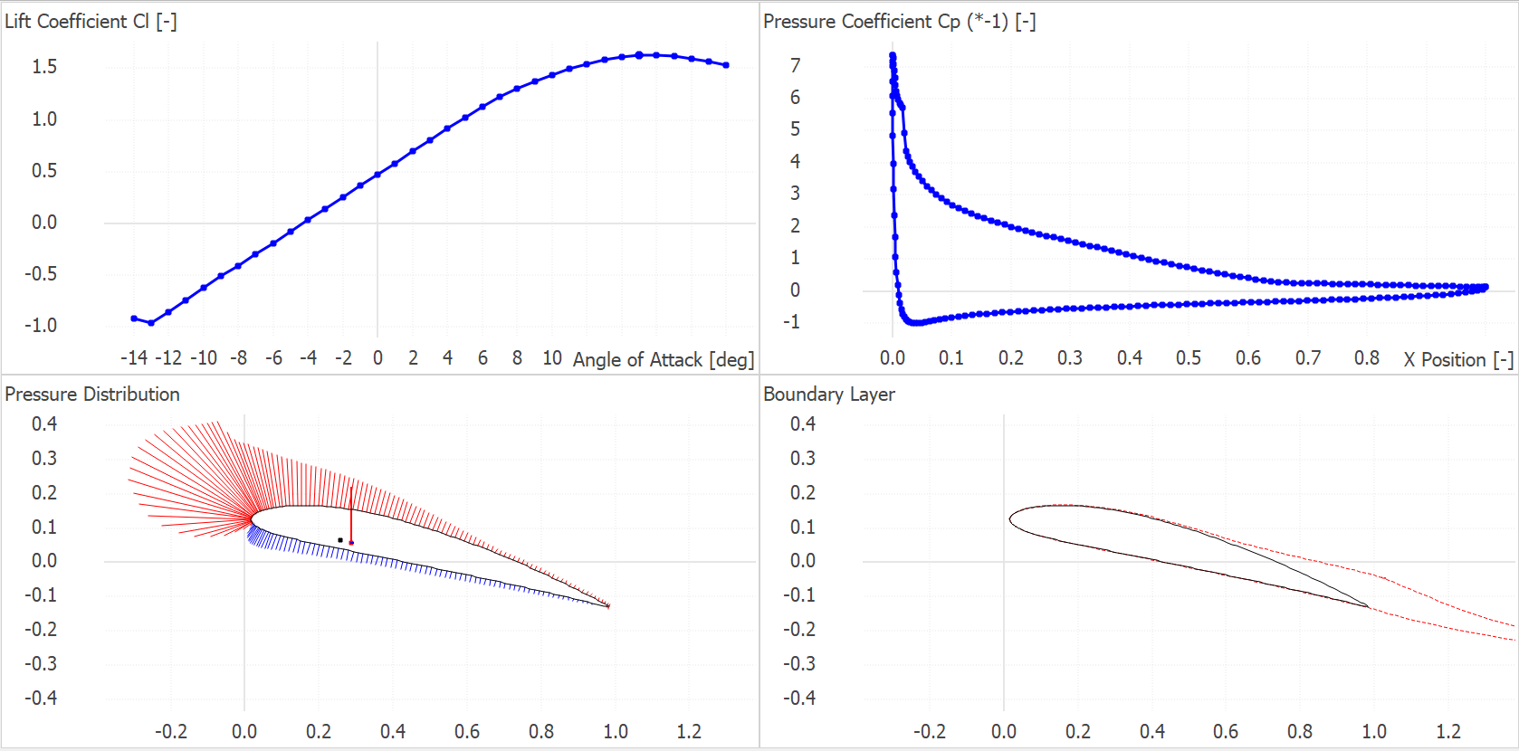
Fig. 67 Operational point data from an airfoil analysis. Top left: Polar plot. Top right: OpPoint plot. Bottom plots: Airfoil visualizations.
Importing Polar Data
Airfoil aerodynamic data can also be imported within the airfoil analysis module by selecting this option in the Polar menu.
Plain Text: The file needs to contain somewhere in the body an array with at least three columns containing: [\(\alpha\), \(C_L\), \(C_D\), (\(C_M\))].
XFOIL: This is a filetype generated by the XFoil solver which contains numerous additional aerodynamic parameters for the airfoil.
NREL (Aerodyn v.13): The Aerodyn v.13
.datformat.QBlade: The polar file
.plrformat of QBlade (see Import and Export of 360 Polars).
It should again be emphasized that polars for the entire \(\alpha\) range are required for an analysis, as such polar import is more practical within the Polar Extrapolation Overview.
Exporting Polar Data
Airfoil polar data generated within the airfoil creation module can be exported for each airfoil either as an XFoil polar file or as an NREL (Aerodyn file simply be selecting the Export Data option from the Polar menu. The option is also available to export all generated airfoil data by selecting Export ALL.