Validation Tests for Morison Equation (ME)

The full Morison Equation (ME) model in QBlade (QB) (see Morison Equation) was validated in a series of test load cases using a semisubmersible substructure model. The load cases were chosen with increasing complexity to make sure the individual modules were working correctly. The test cases include decay tests, regular wave tests and irregular wave tests. Again, the OC4 ME model was considered rigid for these test cases in order to validate the hydrodynamic models.

The results were validated against the open-source aero-hydro-elastic code OpenFAST (OF) 1 (version 2.5.0). The same turbine models and test cases were setup and used in QB and OF. Not all of the hydroelastic modelling capabilities of QB are present in OF. When validating certain hydrodynamic models, the hydrodynamic capabilities of QB were adapted to reflect those of OF to have a better comparison. These modifications are mentioned in the appropriate load cases below.

OC4 Semisubmersible ME Model

The OC4 model was also modelled using the Morison equation only. The geometry of the model is shown in Fig. 158. The Morison equation modelling has the advantage of allowing distributed loading during the simulations and hence enable hydroelastic simulations (see Validation and Examples of Hydroelasticity). As a drawback, the hydrodynamic coefficients for the Morison equation are obtained empirically and are constant for all frequencies. This can lead to modelling inaccuracies compared to the LPMD approach, where the radiation, diffraction and excitation matrices are frequency dependent (see Linear Potential Flow Theory). The hydrodynamic coefficients for the OC4 ME model were taken from the OC4 Report 2 with additional coefficients taken from 3.

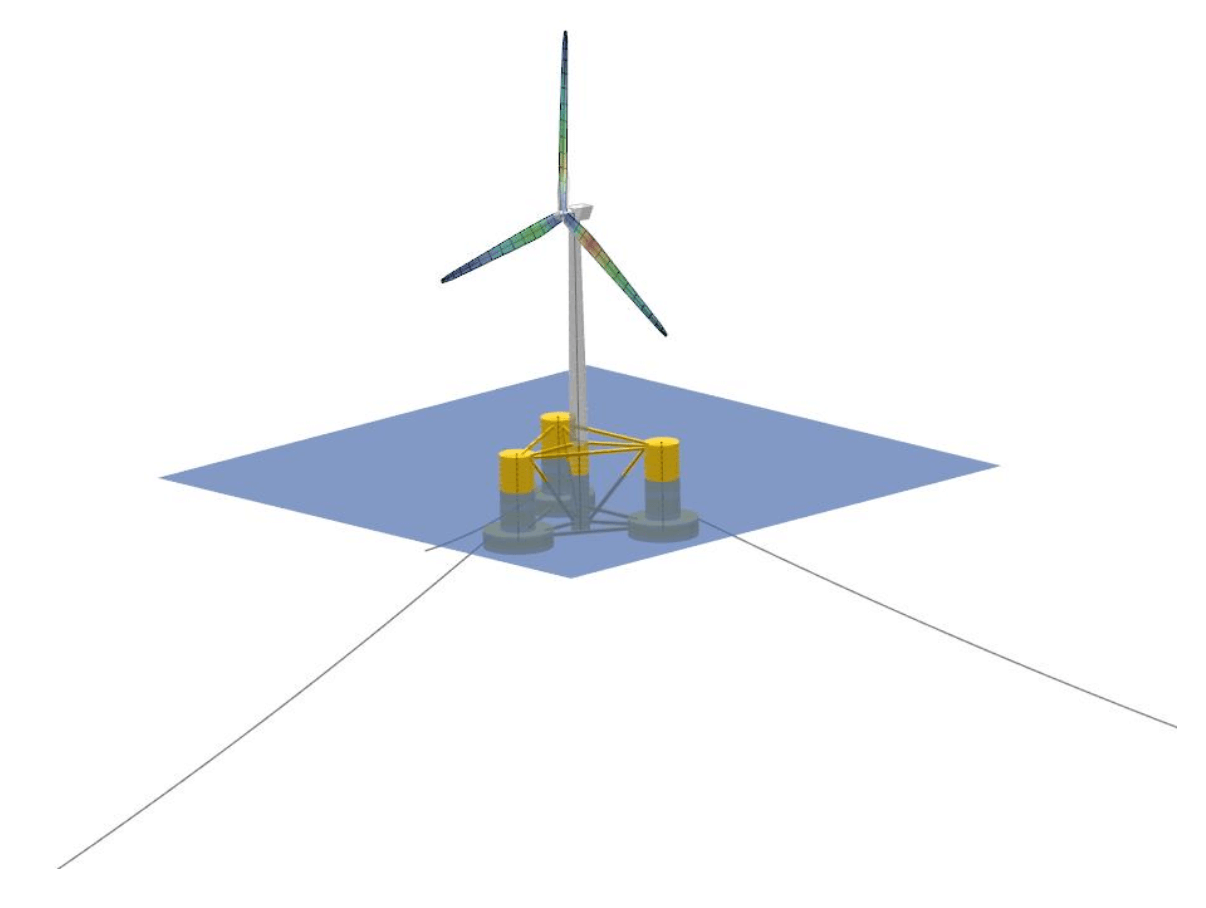
OC4 Model in QB GUI — Fig. 158 The OC4 model displayed in the QB GUI featuring a semisubmersible substructure.

OC4 ME Free Decay Tests

The first test cases were free decay tests with still water. To validate the full Morison equation present in the OC4 ME model, an equivalent ME model was setup in OF. According to the reference 3, the ME model in OF is not able to account for distributed buoyancy. Hence, a linearized buoyancy was used in the OF calculations. This can have a significant effect in the behavior of the substructure when waves are present (see OC4 LPMD Regular Wave Tests).

Fig. 159 to Fig. 161 show the time series of the surge, heave and pitch decay tests. We can see that the models in both codes show a very similar decay behavior. There is a small offset in the heave position due to the different buoyancy models. Also, if we compare with the free decay test of the OC4 LMPD model (see OC4 LPMD Free Decay Tests), we can see that the oscillations damp out more slowly in the decay tests with the OC4 ME model. This is because the OC4 ME model does not have radiation damping forces which act as an additional linear damping term.

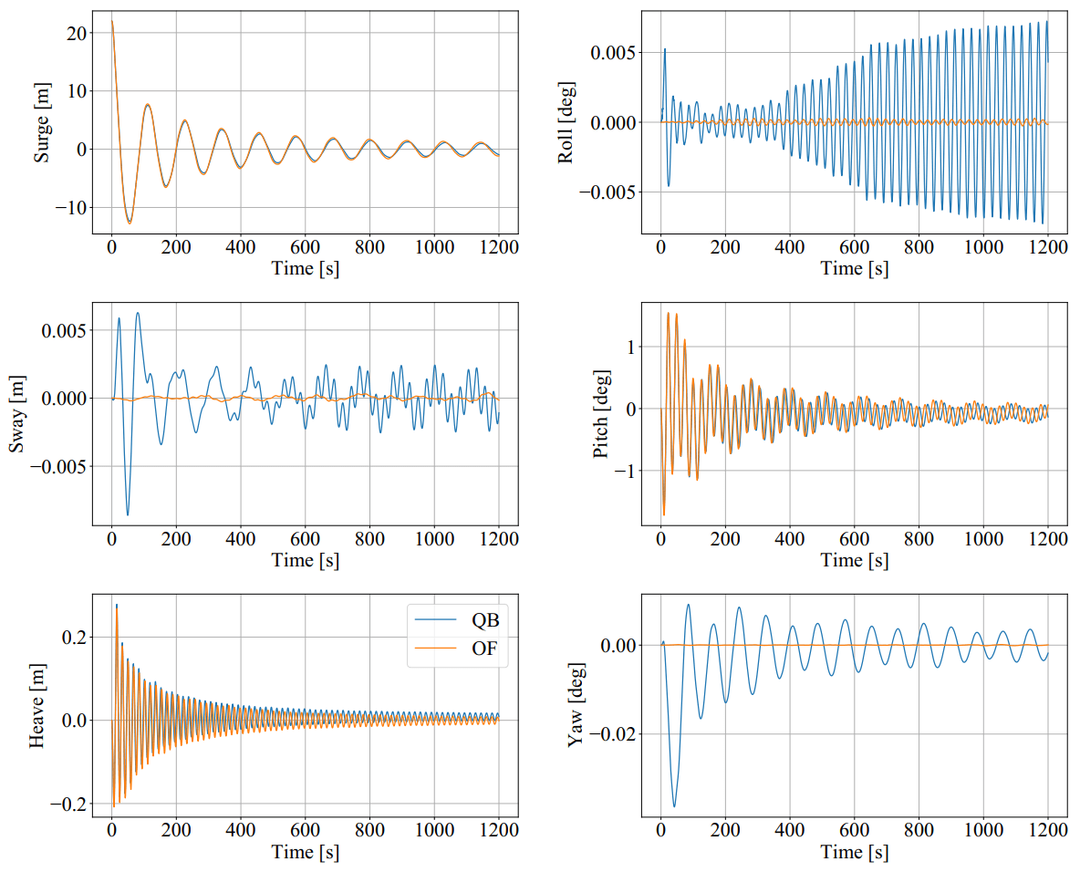
OC4 Model Surge Decay Test — Fig. 159 Time series of the OC4 model surge decay test.

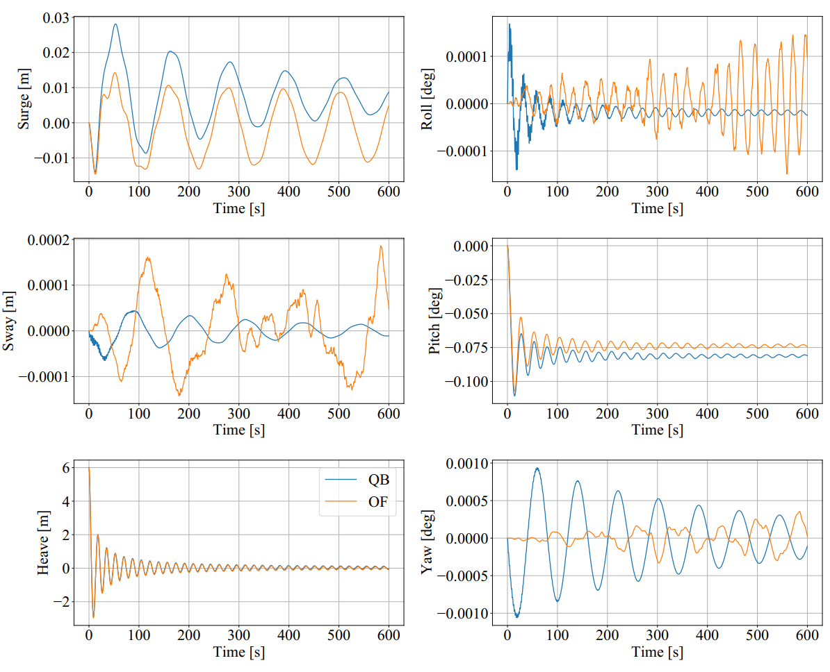
OC4 Model Heave Decay Test — Fig. 160 Time series of the OC4 model heave decay test.

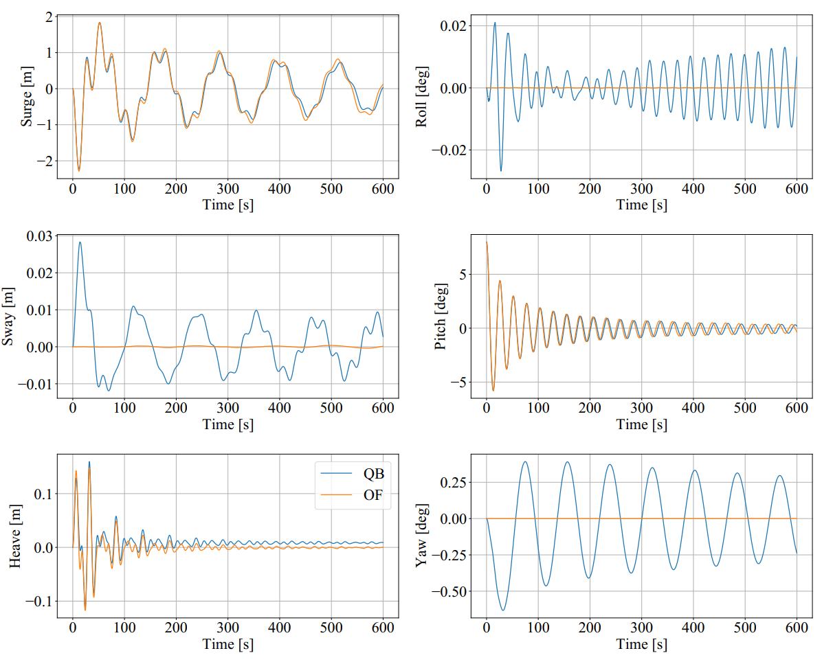
OC4 Model Pitch Decay Test — Fig. 161 Time series of the OC4 model pitch decay test.

We note that the tensions in the mooring system was validated for the OC3 and OC4 models in Validation Tests for Potential Flow Models with Morison Drag (LPMD), so it won’t be repeated here.

Fig. 162 shows the numerical relative values of the eigenfrequencies and damping coefficients of the decay tests for the surge, heave, pitch and yaw degrees of freedom (DOFs). The eigenfrequencies and dampings were obtained according to the procedure presented in 4. The linear damping term was ommited since there is no linear damping present in this model. We can see in this figure that the values for the frequencies and damping coefficients are very similar in both codes. There seems to be a discrepancy in the eigenfrequency of the surge DOF. This difference comes from the method we used to determine the eigenfrequency. For the surge DOF, the numerical value of the eigenfrequency is low and it is therefore close to the frequency resolution we used to determine it. In OF and QB, the peaks in the frequency transform of the signal were shifted in the frequency range by one resolution point. This already accounted for the difference seen in Fig. 162. Visual inspection of Fig. 159 already gives an empirical proof that the frequencies of the surge decay test are very similar.

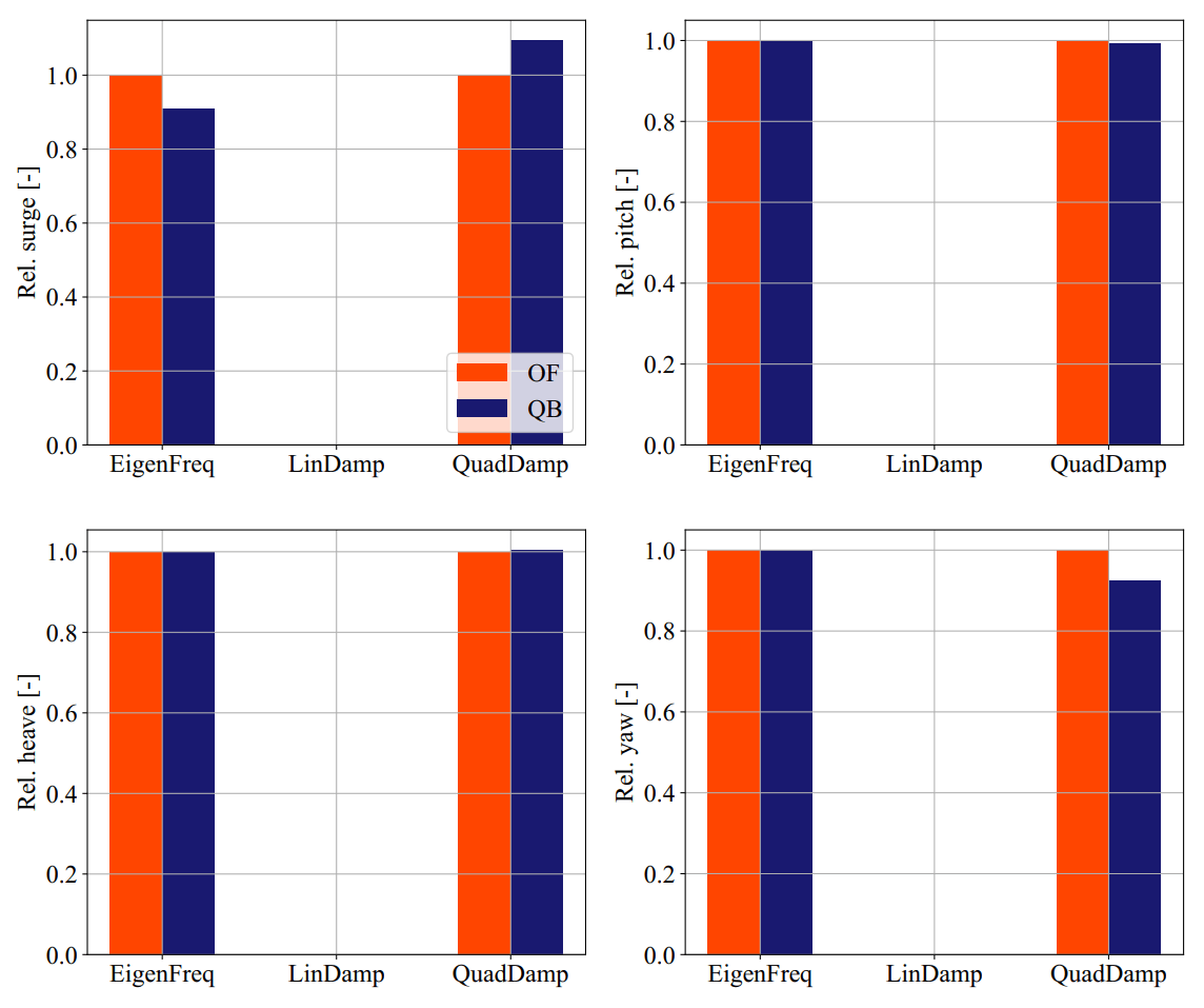
OC4 Model Normalized Frequencies and Dampings — Fig. 162 Normalized eigenfrequencies and damping behaviour of the OC4 model for the considered decay tests.

OC4 ME Regular Wave Tests

The regular wave tests were performed with linear waves for two selected cases. One case had a wave height of \(H\) = 6 m and a period of \(T\) = 10 s. The second case had a wave height of \(H\) = 8 m and a period of \(T\) = 12 s.

For these cases, the OC4 ME was adapted to have a linearized buoyancy model and a linearized mooring system model. Additionally, the wetted surface was considered to go until the mean sea level instead of the local wave elevation (see Modeling Considerations for Morison Elements). This was done to better compare the QB model with the one present in the OF calculations. From test cases presented in Validation Tests for Potential Flow Models with Morison Drag (LPMD), we can consider the buoyancy and mooring models validated. By aligning the modelling considerations between OB and OF, we can better validate the full Morison model developed in QB.

Diffraction forces will play a role for Morison elements that have a diameter larger than a fifth of the wavelength of the incoming wave 5. For the OC4 ME model, this would be relevant for the large base and upper columns if the turbine operates at low sea states 2. In QB, the full Morison model can be extended with the MacCamy-Fuchs correction (MCFC) to take into account the diffraction effects 6.

The regular wave test cases considered three sea states: the first one characterized by \(H\) = 0.67 m and \(T\) = 4.8 s, the second by \(H\) = 6 m and \(T\) = 10 s and the third by \(H\) = 8 m and \(T\) = 12 s. The wave direction was aligned with the positive surge direction. According to 2, the diffraction forces will be relevant for the first sea state.

Fig. 163 to Fig. 165 show the surge, pitch and heave DOFs and the wave elevation for the three regular sea states. We can see in these figures that the results form OF and QB align fairly well in all three sea states. There are some small differences in the heave response in all three cases. When we enable the MacCamy-Fuchs correction in QB, we can see that especially the surge DOF is affected in Fig. 163 and Fig. 164. For the sea state with the smallest wave height, we see the largest differences between the models with and without the MCFC. For larger wave heights (Fig. 164), there are still some differences between the calculations with and without MCFC. These differences practically vanish for the largest wave height case (Fig. 165). This qualitative behavior corresponds to the expected behavior that the MCFC mostly affects sea states where the diameter of the Morison element is comparable to the wave length of the incoming wave.

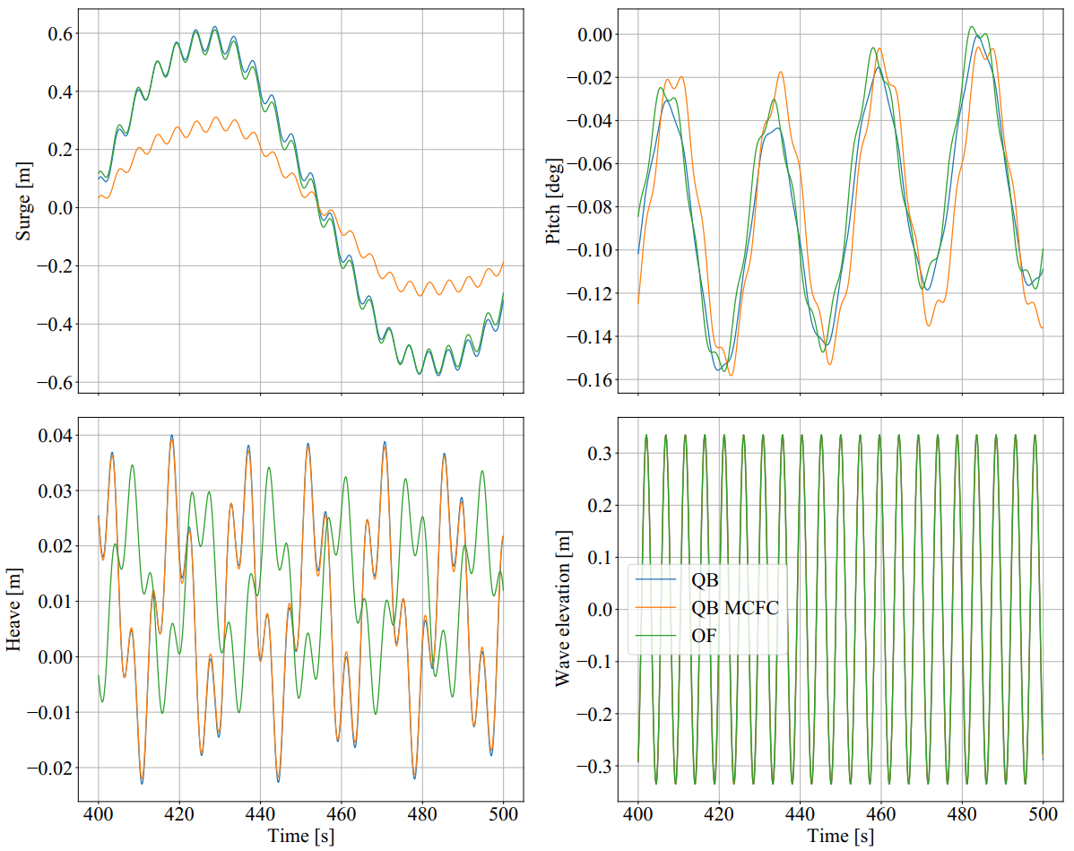
OC4 Regular Wave Test Case 1 — Fig. 163 Relevant DOFs and wave elevation for regular sea state with \(H\) = 0.67 m and \(T\) = 4.8 s. QB MCFC = QB with MacCamy-Fuchs correction.

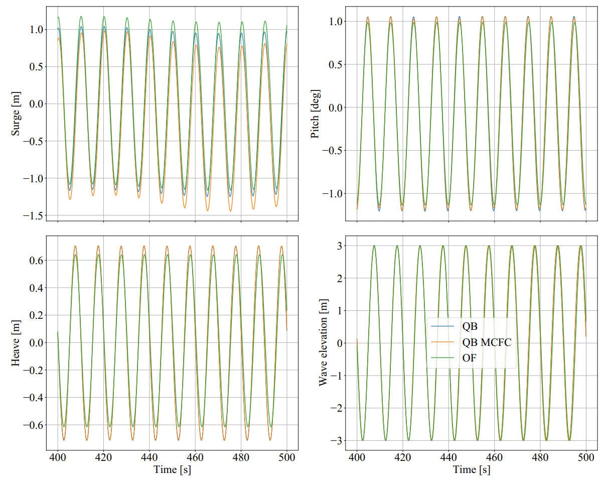
OC4 Regular Wave Test Case 2 — Fig. 164 Relevant DOFs and wave elevation for regular sea state with \(H\) = 6 m and \(T\) = 10 s. QB MCFC = QB with MacCamy-Fuchs correction.

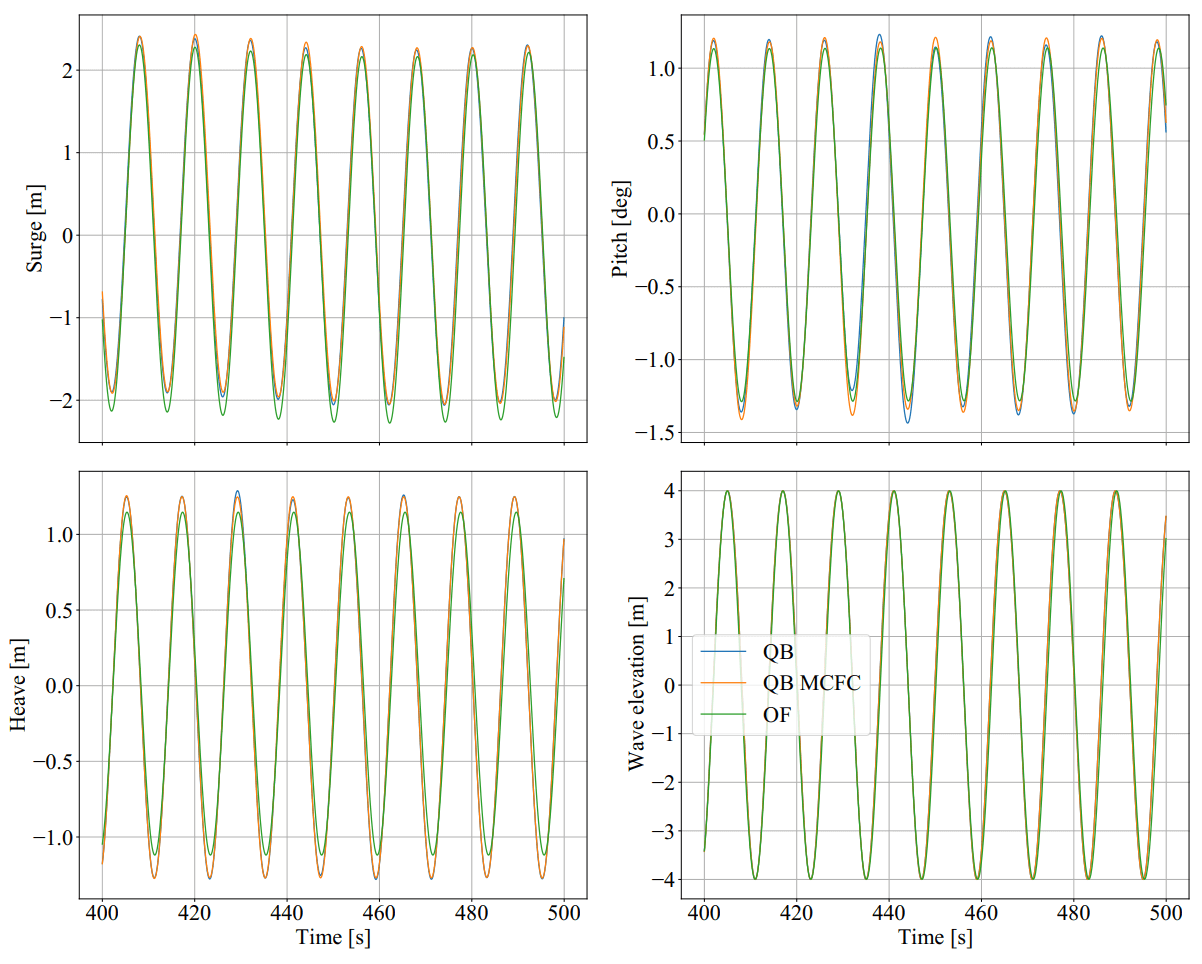
OC4 Regular Wave Test Case 3 — Fig. 165 Relevant DOFs and wave elevation for regular sea state with \(H\) = 8 m and \(T\) = 12 s. QB MCFC = QB with MacCamy-Fuchs correction.

OC4 ME Irregular Wave Tests

The OC4 ME was also tested in sea states with irregular waves and compared to the results from OF simulations. We used six stochastic sea states with a JONSWAP spectrum (\(H_s\) = 6, \(T_p\) = 10 s, \(\gamma\) = 3.3) and compared the averaged PSD of all DOFs. To have a good alignment of the modeling assumptions between QB and OF, we again used a linear buoyancy and a linear mooring model. Also, the wetted surface was assumed to go until the mean sea level and no MCFC was used in the QB simulations. For the irregular wave tests, the wave direction was aligned with the positive surge direction and no aerodynamic loads were considered.

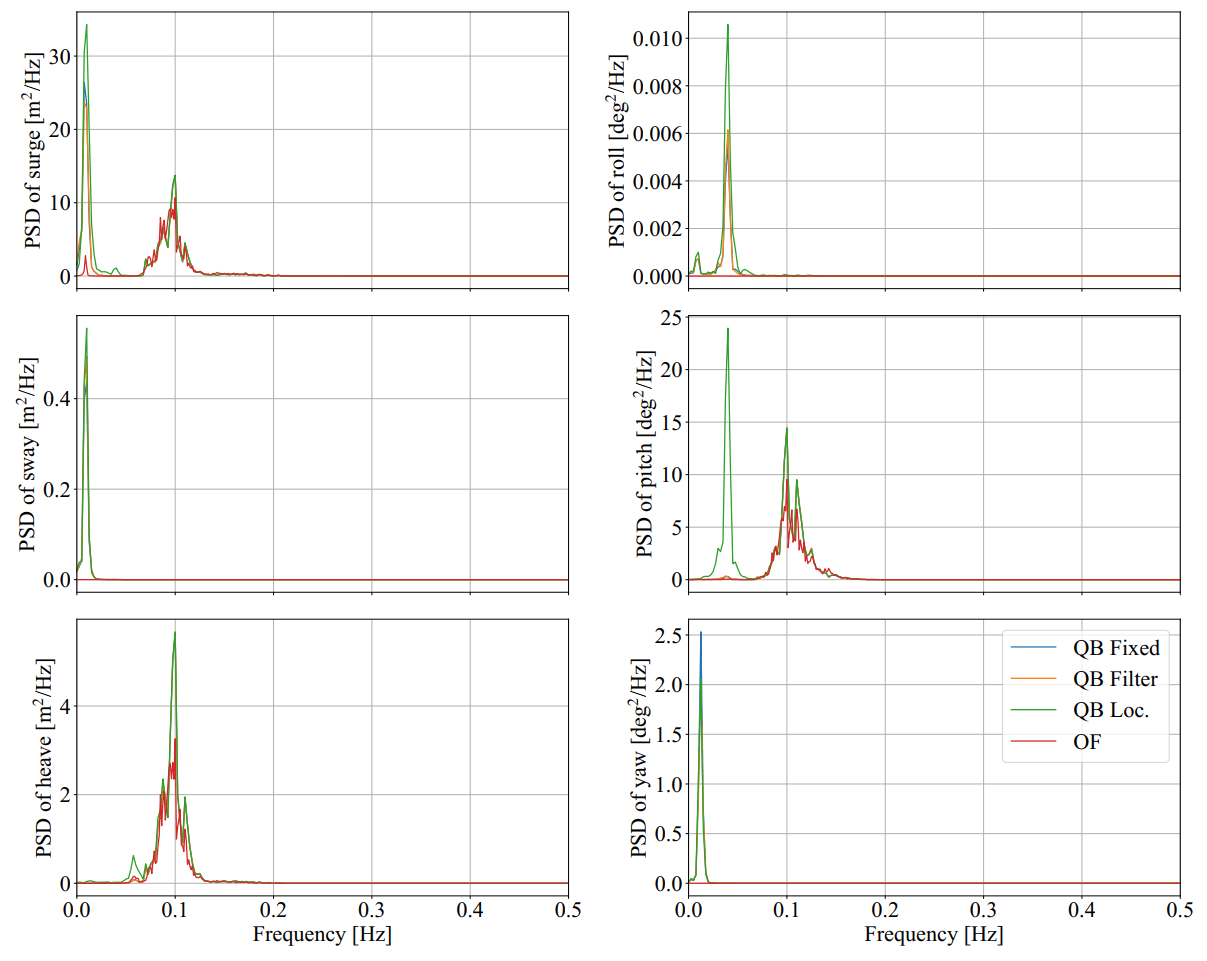
OC4 Irregular Waves tests — Fig. 166 Averaged PSDs of all DOFs of the OC4 ME model for the irregular sea state with \(H_s\) = 6 m, \(T_p\) = 10 s and \(\gamma\) = 3.3.

The comparison was done in a statistical manner by comparing the six-simulation-averaged PSD for the six DOFs. Fig. 166 shows the results of the irregular sea state test cases. We can see that the responses of the OF and QB simulations generally agree well. For the QB simulations, we considered simulations with the three ME implementation options (see Modeling Considerations for Morison Elements). The first option, QB Loc., considered the instantaneous local position of the Morison elements to calculate the water particle kinematics. The second option, QB Filter, considered the low-pass filtered position of the Morison elements to determine the water particle kinematics. The third option, QB Fixed, considered the fixed initial position of the Morison elements for the kinematic calculations. The last option is also implemented in OF 7.

We can see in Fig. 166 that all simulations have a comparable PSD behavior for the wave excitation frequencies (around 0.1 Hz). The higher peaks in the heave and pitch DOFs come from the higher response of the OC4 ME model to wave excitation forces around these frequencies (see e.g. Fig. 164). The strongest differences are seen for the QB Loc. and OF calculations in the low frequency range. The QB Loc. calculations show a peak in the eigenfrequencies of the pitch and surge DOFs while the OF calculations do not. This nonlinear response in pitch disappears for the QB Filter and QB Fixed simulations. It can therefore be attributed to the local instantaneous approach when calculating the water kinematics. The surge DOF still shows a peak in the surge eigenfrequency even when filtered or fixed approach is used for calculating the water kinematics. Further investigation is required to fully understand this phenomenon.

1: OpenFAST. OpenFAST. https://github.com/OpenFAST/openfast, 2021. [Online; accessed 2021-12-07].
2(1,2,3): A. Robertson, J. Jonkman, M. Masciola, H. Song, A. Goupee, A. Coulling, and C. Luan. Definition of the Semisubmersible Floating System for Phase II of OC4. Technical Report TP-5000-60601, NREL, Golden, Colorado, USA, 2014.
3(1,2): F. Wendt, A. Robertson, J. Jonkman, and G. Hayman. Verification of new floating capabilities in fast v8. In 33rd ASME Wind Energy Symposium. 01 2015. doi:10.2514/6.2015-1204.
4: A. Robertson, J. Jonkman, F. Wendt, A. Goupee, and H Dagher. Definition of the OC5 DeepCwind Semisubmersible Floating System. https://a2e.energy.gov/data/oc5/oc5.phase2/attach/oc5.phase2.model.definitionsemisubmersible-floating-system-phase2-oc5-ver15.pdf, 2021. [Online; accessed 2021-11-11].
5: O. M. Faltinsen. Sea Loads on Ships and Offshore Structures. Cambridge University Press, 1993.
6: IEC61400-3-1 Standard. IEC 61400-3-1: Wind Energy Generation Systems - Part 3-1: Design Requirements for fixed offshore wind turbines. Standard, International Electrotechnical Commission, Geneva, Switzerland, 2019.
7: NREL. HydroDyn User Guide and Theory Manual. https://openfast-wave-stretching.readthedocs.io/en/f-wave_stretching/source/user/hydrodyn/#, 2021. [Online; accessed 2021-11-16].